Why xarray?#
xhycom returns xarray Datasets. If you have not used xarray before, this page explains why that is a good thing.
From raw indices to labelled dimensions#
A NumPy array is a grid of numbers. The only way to refer to a location is by its integer position:
arr[0, 5, 100, 200] # what does this mean?
An xarray Dataset wraps the same numbers but gives every axis a name, attaches
coordinate values, and carries metadata. Here is a small toy example with the
same structure as a HYCOM archive — two variables on a (time, k, y, x) grid:
<xarray.Dataset> Size: 1MB
Dimensions:  (time: 12, k: 10, y: 20, x: 30)
Coordinates:
  * time     (time) object 96B 2020-01-01 00:00:00 ... 2020-12-01 00:00:00
  * k        (k) int64 80B 1 2 3 4 5 6 7 8 9 10
    dens     (k) float64 80B 26.0 26.22 26.44 26.67 ... 27.33 27.56 27.78 28.0
    lon      (y, x) float64 5kB -10.0 -9.31 -8.621 -7.931 ... 8.621 9.31 10.0
    lat      (y, x) float64 5kB 50.0 50.0 50.0 50.0 50.0 ... 70.0 70.0 70.0 70.0
Dimensions without coordinates: y, x
Data variables:
    temp     (time, k, y, x) float64 576kB 5.377 4.604 6.921 ... 10.27 5.168
    salin    (time, k, y, x) float64 576kB 32.44 34.55 34.07 ... 35.24 35.59
    srfhgt   (time, y, x) float64 58kB -6.647e+03 -635.5 ... 5.214e+03
Attributes:
description: Toy ocean dataset (same structure as a HYCOM archive)Click the icons on the right of each row to expand coordinates and attributes. Notice:
Every axis has a name —
time,k,y,x— not just an integer position.lonandlatare 2-D curvilinear coordinates: they live on the(y, x)grid, just like a real ocean model on a non-rectangular grid.densgives each vertical layer a physical label (target sigma-2 density), so you can writeds["temp"].sel(dens=27.0, method="nearest")instead ofarr[:, 5, :, :].Every variable carries CF-style attributes (
long_name,units) that appear automatically in plot labels.
Coordinates travel with the data#
Operations on an xarray object preserve coordinates automatically. Slice a layer, take a time mean, compute an anomaly — the result always knows where it is:
# Select surface layer and take a time mean — coordinates are preserved automatically
sst_mean = ds["temp"].isel(k=0).mean("time")
sst_mean
<xarray.DataArray 'temp' (y: 20, x: 30)> Size: 5kB
array([[4.49613298, 4.82798084, 3.30136389, 5.24302273, 5.81710217,
        5.25808985, 6.22346355, 4.19645876, 5.88739858, 4.76628531,
        4.88347417, 4.60155376, 4.66092057, 5.42924823, 4.92985383,
        4.96666037, 6.37363088, 4.76892471, 5.13895149, 5.85705093,
        4.41965531, 5.07794453, 4.49980205, 5.90155666, 5.95883614,
        5.99369286, 3.02222098, 4.84304793, 3.47142542, 4.71514191],
       [4.22540109, 5.02764166, 3.89466327, 5.99957853, 4.04206223,
        5.17582447, 5.44023634, 5.92491076, 5.60205596, 4.56262881,
        5.09245145, 5.18176807, 4.86460777, 4.29143486, 5.22939139,
        6.09650067, 5.71176562, 4.95496655, 4.96653507, 5.60478466,
        4.80325627, 5.39526157, 5.96105618, 5.0385708 , 4.38118054,
        3.76238749, 5.47089344, 4.44839623, 4.24289887, 3.65937114],
       [4.20766584, 4.51441481, 4.4486331 , 2.87743268, 4.48701748,
        4.5780106 , 5.45851012, 5.95721997, 5.58286811, 4.44527348,
        6.59369433, 4.60638076, 4.65108344, 5.46039457, 5.18542486,
        5.29270798, 3.58552177, 4.71932838, 6.18540324, 4.5579556 ,
        5.6491876 , 4.86902926, 4.33864119, 5.74451508, 4.75044865,
        3.72659193, 5.18721568, 5.11248662, 5.29448538, 6.02935357],
       [5.48034114, 4.44975344, 4.60267035, 4.80793269, 5.37670629,
        4.563093  , 4.66433469, 5.35726249, 3.78690324, 5.61068043,
...
        3.94610453, 3.18401636, 3.71646145, 4.43729776, 5.5073521 ,
        5.18690552, 5.28329469, 4.41689295, 6.45973727, 4.62682623],
       [4.52041382, 6.39514059, 4.41282125, 5.5275527 , 6.56798967,
        5.41445805, 5.47712146, 5.93748723, 4.81265524, 5.51234996,
        5.44742824, 4.91465904, 3.42891314, 4.22864721, 3.82372354,
        6.26377656, 4.86902194, 5.33199637, 5.32325795, 5.49784115,
        5.39495439, 5.81019206, 5.20906634, 6.26609038, 4.4266159 ,
        5.237327  , 3.67216623, 4.88932123, 3.40165156, 3.57099877],
       [3.34752729, 6.07626989, 4.40935618, 3.52280523, 6.07465843,
        3.40645781, 2.78146854, 3.42403301, 4.92466896, 5.11261783,
        5.33269822, 4.17501649, 5.09337563, 5.5027163 , 3.97657581,
        5.61419913, 5.61749952, 6.53217472, 4.25067714, 6.39623669,
        5.66717638, 4.8257111 , 3.842357  , 4.59043952, 5.51492238,
        5.43796308, 7.66401062, 4.11364749, 4.66576816, 3.8071525 ],
       [5.03941047, 6.31086418, 5.72736335, 4.81302109, 3.72079676,
        6.39029313, 5.10725839, 4.33199012, 2.83002489, 4.96997614,
        4.94872889, 3.96301739, 6.10587176, 4.35128376, 4.18382449,
        5.93445922, 5.44718828, 5.21718118, 4.81585582, 6.73073586,
        5.28021211, 4.77759747, 5.64729846, 4.49536223, 4.58174361,
        6.39118856, 3.42504117, 3.6984635 , 3.49841477, 5.83300251]])
Coordinates:
    lon      (y, x) float64 5kB -10.0 -9.31 -8.621 -7.931 ... 8.621 9.31 10.0
    lat      (y, x) float64 5kB 50.0 50.0 50.0 50.0 50.0 ... 70.0 70.0 70.0 70.0
    k        int64 8B 1
    dens     float64 8B 26.0
Dimensions without coordinates: y, x
Attributes:
    long_name:  sea water potential temperature
units: degCsst_mean still knows its lon, lat, k, and dens — they were not discarded
by .isel() or .mean(). With raw NumPy you would have to carry those arrays
separately and reattach them after every operation.
Plotting just works#
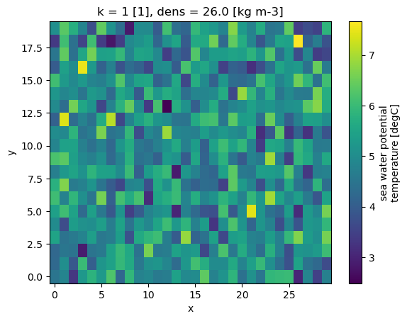
Because coordinates are embedded in the data, xarray’s .plot() method
automatically labels axes, titles, and colourbars:
sst_mean.plot()
<matplotlib.collections.QuadMesh at 0x146378f7d150>
Note
The data above is randomly generated for illustration purposes. See the quick start for plots of real HYCOM output.
With NumPy + Matplotlib you would need to pass lon and lat explicitly to
pcolormesh, set axis labels by hand, and add the colourbar yourself.
Larger-than-memory data via Dask#
xarray integrates with Dask to represent datasets that are far larger than available RAM. Instead of reading data immediately, xarray builds a computation graph: a recipe for what to do when you finally ask for the result.
                          open_mfdataset(..., chunks={"time": 1})
                          ┌─────────────────────────────────────┐
30 years of .ab files ───►│  Dask-backed xr.Dataset             │
(~1 TB on disk)           │  in memory: ~100 MB (graph only)    │
                          └───────────────┬─────────────────────┘
                                          │  .isel(k=0).mean("time")
                                          ▼
                          ┌─────────────────────────────────────┐
                          │  lazy computation graph             │
                          │  (still nothing read from disk)     │
                          └───────────────┬─────────────────────┘
                                          │  .compute()
                                          ▼
                          ┌─────────────────────────────────────┐
                          │  result: (y, x) NumPy array         │
                          │  only the needed chunks were read   │
                          └─────────────────────────────────────┘
This is what makes it possible to compute a 30-year mean SST on a laptop without running out of memory.
The broader ecosystem#
An xarray Dataset plugs into a large ecosystem of scientific Python tools without any glue code:
Task |
Tool |
|---|---|
Interactive maps |
|
Parallel computation |
|
Cloud-optimised storage |
|
Regridding |
|
Statistics |
|
Filtering |
Because xhycom returns standard xarray objects, all of these work on HYCOM output immediately — no adapters or format conversions required.