Lazy loading & chunking#
This notebook shows how to open large multi-year HYCOM archives without loading field data into memory, explains why the task graph can itself become expensive, and presents two practical remedies.
We use the memory_profiler extension throughout:
%%timereports wall-clock and CPU time.%%memitreports peak memory and increment (memory added on top of what was already in use).
import xhycom
Set the paths below to point at your data before running.
GRID_PATH = "/cluster/home/nlo043/NERSC-HYCOM-CICE/TP2a0.10/topo/regional.grid"
BATHY_PATH = "/cluster/home/nlo043/NERSC-HYCOM-CICE/TP2a0.10/topo/depth_TP2a0.10_01"
DATA_PATH = "/nird/datalake/NS9481K/shuang/TP2_output/expt_02.8/"  # directory containing archv.*.ab or archm.*.ab
Open a time series#
Pass a directory or a glob pattern and xhycom discovers all matching .ab file pairs, parses their .b headers, and returns a single Dataset with a time dimension spanning every snapshot in chronological order.
To understand the memory and time cost of each approach, we use the memory_profiler extension:
%%timereports wall-clock and CPU time for the cell.%%memitreports peak memory (the high-water mark reached during the cell) and increment (how much extra memory was allocated on top of what was already in use before the cell ran).
We start by opening the first 9 daily files of 2020 without chunking, so all field data is read eagerly into RAM.
%load_ext memory_profiler
%%time
%%memit
ds = xhycom.open_mfdataset(DATA_PATH + "archm.2020_00*", grid=GRID_PATH)
peak memory: 55212.14 MiB, increment: 55097.10 MiB
CPU times: user 15.3 s, sys: 7.5 s, total: 22.8 s
Wall time: 1min 25s
The output tells us two things:
Increment: ~54 GB — xhycom read every
.abinary file in full and allocated one array per variable per time step. With only 9 files and 83 variables this is already enormous; a full year would consume hundreds of GB, and a multi-decade archive would be completely unworkable.Wall time: ~26 s — the call blocked for 26 seconds while all that data was transferred from disk into RAM.
Note
%%time and %%memit are optional. Remove them from any cell if you are not interested in the profiling output — they have no effect on the returned data.
ds
<xarray.Dataset> Size: 29GB
Dimensions:     (time: 9, y: 380, x: 400, k: 50, ki: 51)
Coordinates:
  * time        (time) object 72B 2020-01-01 00:00:00 ... 2020-01-09 00:00:00
    lon         (y, x) float64 1MB -94.75 -94.58 -94.42 ... 99.09 98.95 98.82
    lat         (y, x) float64 1MB 39.06 39.16 39.26 39.36 ... 56.39 56.29 56.2
    lon_u       (y, x) float64 1MB -94.83 -94.67 -94.5 ... 99.16 99.02 98.89
    lat_u       (y, x) float64 1MB 39.01 39.11 39.21 39.31 ... 56.43 56.34 56.25
    lon_v       (y, x) float64 1MB -94.68 -94.52 -94.35 ... 99.0 98.87 98.74
    lat_v       (y, x) float64 1MB 38.99 39.09 39.19 39.29 ... 56.43 56.33 56.24
  * k           (k) int64 400B 1 2 3 4 5 6 7 8 9 ... 42 43 44 45 46 47 48 49 50
    dens        (k) float64 400B 0.1 0.2 0.3 0.4 0.5 ... 28.09 28.1 28.11 28.12
  * ki          (ki) int64 408B 0 1 2 3 4 5 6 7 8 ... 42 43 44 45 46 47 48 49 50
Dimensions without coordinates: y, x
Data variables: (12/83)
    montg1      (time, y, x) float64 11MB nan nan nan nan ... nan nan nan nan
    srfhgt      (time, y, x) float64 11MB nan nan nan nan ... nan nan nan nan
    oneta       (time, y, x) float64 11MB nan nan nan nan ... nan nan nan nan
    surflx      (time, y, x) float64 11MB nan nan nan nan ... nan nan nan nan
    wtrflx      (time, y, x) float64 11MB nan nan nan nan ... nan nan nan nan
    salflx      (time, y, x) float64 11MB nan nan nan nan ... nan nan nan nan
    ...          ...
    CO2_wind    (time, y, x) float64 11MB nan nan nan nan ... nan nan nan nan
    ECO_bots    (time, y, x) float64 11MB nan nan nan nan ... nan nan nan nan
    surface__1  (time, y, x) float64 11MB nan nan nan nan ... nan nan nan nan
    surface__2  (time, y, x) float64 11MB nan nan nan nan ... nan nan nan nan
    si_u        (time, y, x) float64 11MB nan nan nan nan ... nan nan nan nan
    si_v        (time, y, x) float64 11MB nan nan nan nan ... nan nan nan nan
Attributes:
    iversn:   23
    iexpt:    28
yrflag: 3- time: 9
- y: 380
- x: 400
- k: 50
- ki: 51
- time(time)object2020-01-01 00:00:00 ... 2020-01-...
- long_name :
- time
- axis :
- T
array([cftime.DatetimeGregorian(2020, 1, 1, 0, 0, 0, 0, has_year_zero=False), cftime.DatetimeGregorian(2020, 1, 2, 0, 0, 0, 0, has_year_zero=False), cftime.DatetimeGregorian(2020, 1, 3, 0, 0, 0, 0, has_year_zero=False), cftime.DatetimeGregorian(2020, 1, 4, 0, 0, 0, 0, has_year_zero=False), cftime.DatetimeGregorian(2020, 1, 5, 0, 0, 0, 0, has_year_zero=False), cftime.DatetimeGregorian(2020, 1, 6, 0, 0, 0, 0, has_year_zero=False), cftime.DatetimeGregorian(2020, 1, 7, 0, 0, 0, 0, has_year_zero=False), cftime.DatetimeGregorian(2020, 1, 8, 0, 0, 0, 0, has_year_zero=False), cftime.DatetimeGregorian(2020, 1, 9, 0, 0, 0, 0, has_year_zero=False)], dtype=object) - lon(y, x)float64-94.75 -94.58 ... 98.95 98.82
- long_name :
- longitude (T-point)
- units :
- degrees_east
- standard_name :
- longitude
array([[ -94.74750519, -94.58249664, -94.41687775, ..., 5.86695623, 6.06488323, 6.26205826], [ -94.87778473, -94.71282959, -94.5472641 , ..., 5.99605846, 6.1941061 , 6.391397 ], [ -95.00868225, -94.84378815, -94.67826843, ..., 6.12591982, 6.32408571, 6.5214901 ], ..., [-173.207901 , -173.30162048, -173.39605713, ..., 98.75035858, 98.61607361, 98.48277283], [-173.36988831, -173.46382141, -173.55848694, ..., 98.92017365, 98.78582764, 98.65245819], [-173.53115845, -173.62532043, -173.72019958, ..., 99.08900452, 98.95459747, 98.82115936]], shape=(380, 400)) - lat(y, x)float6439.06 39.16 39.26 ... 56.29 56.2
- long_name :
- latitude (T-point)
- units :
- degrees_north
- standard_name :
- latitude
array([[39.05597305, 39.15685272, 39.25762558, ..., 43.83851242, 43.74554825, 43.65235138], [39.18373108, 39.28490067, 39.38597107, ..., 43.98142242, 43.888134 , 43.79462051], [39.31121063, 39.41267776, 39.51403809, ..., 44.12407684, 44.03046799, 43.93662643], ..., [51.74200058, 51.84247589, 51.94287109, ..., 56.53710175, 56.44309616, 56.34889603], [51.68408203, 51.78424835, 51.88433075, ..., 56.46269226, 56.36904907, 56.27520752], [51.62594986, 51.72580338, 51.82557678, ..., 56.3881073 , 56.29482269, 56.20133972]], shape=(380, 400)) - lon_u(y, x)float64-94.83 -94.67 -94.5 ... 99.02 98.89
- long_name :
- longitude (U-point)
- units :
- degrees_east
array([[ -94.82977295, -94.66507721, -94.49976349, ..., 5.76771021, 5.96601391, 6.16356468], [ -94.9600296 , -94.79538727, -94.63012695, ..., 5.89674997, 6.09517717, 6.2928462 ], [ -95.09089661, -94.92630768, -94.7611084 , ..., 6.02655029, 6.22509813, 6.42288303], ..., [-173.16131592, -173.25466919, -173.34875488, ..., 98.81787109, 98.68309021, 98.54930115], [-173.32318115, -173.41676331, -173.51106262, ..., 98.98771667, 98.85287476, 98.71901703], [-173.48432922, -173.57815552, -173.67266846, ..., 99.15657806, 99.02167511, 98.88775635]], shape=(380, 400)) - lat_u(y, x)float6439.01 39.11 39.21 ... 56.34 56.25
- long_name :
- latitude (U-point)
- units :
- degrees_north
array([[39.00549698, 39.10642624, 39.2072525 , ..., 43.88490677, 43.79206085, 43.69897842], [39.13310623, 39.23432922, 39.33544922, ..., 44.02797699, 43.93480682, 43.84140778], [39.26044464, 39.36195755, 39.46337128, ..., 44.17079163, 44.07730103, 43.98357391], ..., [51.69173431, 51.79224777, 51.89268494, ..., 56.58403015, 56.49012375, 56.39601898], [51.63396835, 51.73417664, 51.83430099, ..., 56.50944138, 56.41589737, 56.32215118], [51.57598877, 51.67588806, 51.77569962, ..., 56.43467712, 56.3414917 , 56.24810791]], shape=(380, 400)) - lon_v(y, x)float64-94.68 -94.52 ... 98.87 98.74
- long_name :
- longitude (V-point)
- units :
- degrees_east
array([[ -94.6825943 , -94.51755524, -94.35191345, ..., 5.8026886 , 6.00055408, 6.19766998], [ -94.81256866, -94.64758301, -94.481987 , ..., 5.9314127 , 6.12940025, 6.32663393], [ -94.94315338, -94.77822876, -94.61268616, ..., 6.06089401, 6.25900126, 6.4563489 ], ..., [-173.12664795, -173.22024536, -173.3145752 , ..., 98.66507721, 98.53083038, 98.39756775], [-173.28898621, -173.3828125 , -173.47735596, ..., 98.83538818, 98.70107269, 98.56773376], [-173.4506073 , -173.54466248, -173.63943481, ..., 99.00471497, 98.87033081, 98.73693085]], shape=(380, 400)) - lat_v(y, x)float6438.99 39.09 39.19 ... 56.33 56.24
- long_name :
- latitude (V-point)
- units :
- degrees_north
array([[38.99199295, 39.09272385, 39.19335175, ..., 43.76696396, 43.67416 , 43.58112335], [39.11988831, 39.22091293, 39.32183075, ..., 43.90999985, 43.81687546, 43.72351837], [39.24750519, 39.34882355, 39.45003891, ..., 44.05278015, 43.95933151, 43.86565399], ..., [51.77088165, 51.87150955, 51.97205734, ..., 56.57423782, 56.48004913, 56.38566971], [51.71306992, 51.81338882, 51.91362762, ..., 56.49991989, 56.4060936 , 56.31207275], [51.65504074, 51.75505447, 51.85498047, ..., 56.42542267, 56.33195877, 56.23829651]], shape=(380, 400)) - k(k)int641 2 3 4 5 6 7 ... 45 46 47 48 49 50
- long_name :
- layer index
- units :
- 1
- axis :
- Z
array([ 1, 2, 3, 4, 5, 6, 7, 8, 9, 10, 11, 12, 13, 14, 15, 16, 17, 18, 19, 20, 21, 22, 23, 24, 25, 26, 27, 28, 29, 30, 31, 32, 33, 34, 35, 36, 37, 38, 39, 40, 41, 42, 43, 44, 45, 46, 47, 48, 49, 50]) - dens(k)float640.1 0.2 0.3 ... 28.1 28.11 28.12
- long_name :
- target sigma-2 layer density
- units :
- kg m-3
array([ 0.1 , 0.2 , 0.3 , 0.4 , 0.5 , 0.6 , 0.7 , 0.8 , 0.9 , 1. , 24.05, 25.72, 26.4 , 26.9 , 27.13, 27.19, 27.25, 27.29, 27.34, 27.42, 27.5 , 27.56, 27.63, 27.66, 27.69, 27.72, 27.74, 27.76, 27.78, 27.8 , 27.82, 27.85, 27.87, 27.9 , 27.93, 27.95, 27.97, 27.99, 28.01, 28.02, 28.03, 28.04, 28.05, 28.06, 28.07, 28.08, 28.09, 28.1 , 28.11, 28.12]) - ki(ki)int640 1 2 3 4 5 6 ... 45 46 47 48 49 50
- long_name :
- layer interface index
- units :
- 1
- axis :
- Z
array([ 0,  1,  2,  3,  4,  5,  6,  7,  8,  9, 10, 11, 12, 13, 14, 15, 16, 17,
       18, 19, 20, 21, 22, 23, 24, 25, 26, 27, 28, 29, 30, 31, 32, 33, 34, 35,
       36, 37, 38, 39, 40, 41, 42, 43, 44, 45, 46, 47, 48, 49, 50])
- montg1(time, y, x)float64nan nan nan nan ... nan nan nan nan
- long_name :
- Montgomery potential
- units :
- m2 s-2
array([[[nan, nan, nan, ..., nan, nan, nan], [nan, nan, nan, ..., nan, nan, nan], [nan, nan, nan, ..., nan, nan, nan], ..., [nan, nan, nan, ..., nan, nan, nan], [nan, nan, nan, ..., nan, nan, nan], [nan, nan, nan, ..., nan, nan, nan]], [[nan, nan, nan, ..., nan, nan, nan], [nan, nan, nan, ..., nan, nan, nan], [nan, nan, nan, ..., nan, nan, nan], ..., [nan, nan, nan, ..., nan, nan, nan], [nan, nan, nan, ..., nan, nan, nan], [nan, nan, nan, ..., nan, nan, nan]], [[nan, nan, nan, ..., nan, nan, nan], [nan, nan, nan, ..., nan, nan, nan], [nan, nan, nan, ..., nan, nan, nan], ..., ... ..., [nan, nan, nan, ..., nan, nan, nan], [nan, nan, nan, ..., nan, nan, nan], [nan, nan, nan, ..., nan, nan, nan]], [[nan, nan, nan, ..., nan, nan, nan], [nan, nan, nan, ..., nan, nan, nan], [nan, nan, nan, ..., nan, nan, nan], ..., [nan, nan, nan, ..., nan, nan, nan], [nan, nan, nan, ..., nan, nan, nan], [nan, nan, nan, ..., nan, nan, nan]], [[nan, nan, nan, ..., nan, nan, nan], [nan, nan, nan, ..., nan, nan, nan], [nan, nan, nan, ..., nan, nan, nan], ..., [nan, nan, nan, ..., nan, nan, nan], [nan, nan, nan, ..., nan, nan, nan], [nan, nan, nan, ..., nan, nan, nan]]], shape=(9, 380, 400)) - srfhgt(time, y, x)float64nan nan nan nan ... nan nan nan nan
- long_name :
- sea surface height
- units :
- Pa
array([[[nan, nan, nan, ..., nan, nan, nan], [nan, nan, nan, ..., nan, nan, nan], [nan, nan, nan, ..., nan, nan, nan], ..., [nan, nan, nan, ..., nan, nan, nan], [nan, nan, nan, ..., nan, nan, nan], [nan, nan, nan, ..., nan, nan, nan]], [[nan, nan, nan, ..., nan, nan, nan], [nan, nan, nan, ..., nan, nan, nan], [nan, nan, nan, ..., nan, nan, nan], ..., [nan, nan, nan, ..., nan, nan, nan], [nan, nan, nan, ..., nan, nan, nan], [nan, nan, nan, ..., nan, nan, nan]], [[nan, nan, nan, ..., nan, nan, nan], [nan, nan, nan, ..., nan, nan, nan], [nan, nan, nan, ..., nan, nan, nan], ..., ... ..., [nan, nan, nan, ..., nan, nan, nan], [nan, nan, nan, ..., nan, nan, nan], [nan, nan, nan, ..., nan, nan, nan]], [[nan, nan, nan, ..., nan, nan, nan], [nan, nan, nan, ..., nan, nan, nan], [nan, nan, nan, ..., nan, nan, nan], ..., [nan, nan, nan, ..., nan, nan, nan], [nan, nan, nan, ..., nan, nan, nan], [nan, nan, nan, ..., nan, nan, nan]], [[nan, nan, nan, ..., nan, nan, nan], [nan, nan, nan, ..., nan, nan, nan], [nan, nan, nan, ..., nan, nan, nan], ..., [nan, nan, nan, ..., nan, nan, nan], [nan, nan, nan, ..., nan, nan, nan], [nan, nan, nan, ..., nan, nan, nan]]], shape=(9, 380, 400)) - oneta(time, y, x)float64nan nan nan nan ... nan nan nan nan
- long_name :
- free surface elevation
- units :
- m
array([[[nan, nan, nan, ..., nan, nan, nan], [nan, nan, nan, ..., nan, nan, nan], [nan, nan, nan, ..., nan, nan, nan], ..., [nan, nan, nan, ..., nan, nan, nan], [nan, nan, nan, ..., nan, nan, nan], [nan, nan, nan, ..., nan, nan, nan]], [[nan, nan, nan, ..., nan, nan, nan], [nan, nan, nan, ..., nan, nan, nan], [nan, nan, nan, ..., nan, nan, nan], ..., [nan, nan, nan, ..., nan, nan, nan], [nan, nan, nan, ..., nan, nan, nan], [nan, nan, nan, ..., nan, nan, nan]], [[nan, nan, nan, ..., nan, nan, nan], [nan, nan, nan, ..., nan, nan, nan], [nan, nan, nan, ..., nan, nan, nan], ..., ... ..., [nan, nan, nan, ..., nan, nan, nan], [nan, nan, nan, ..., nan, nan, nan], [nan, nan, nan, ..., nan, nan, nan]], [[nan, nan, nan, ..., nan, nan, nan], [nan, nan, nan, ..., nan, nan, nan], [nan, nan, nan, ..., nan, nan, nan], ..., [nan, nan, nan, ..., nan, nan, nan], [nan, nan, nan, ..., nan, nan, nan], [nan, nan, nan, ..., nan, nan, nan]], [[nan, nan, nan, ..., nan, nan, nan], [nan, nan, nan, ..., nan, nan, nan], [nan, nan, nan, ..., nan, nan, nan], ..., [nan, nan, nan, ..., nan, nan, nan], [nan, nan, nan, ..., nan, nan, nan], [nan, nan, nan, ..., nan, nan, nan]]], shape=(9, 380, 400)) - surflx(time, y, x)float64nan nan nan nan ... nan nan nan nan
- long_name :
- net surface heat flux
- units :
- W m-2
array([[[nan, nan, nan, ..., nan, nan, nan], [nan, nan, nan, ..., nan, nan, nan], [nan, nan, nan, ..., nan, nan, nan], ..., [nan, nan, nan, ..., nan, nan, nan], [nan, nan, nan, ..., nan, nan, nan], [nan, nan, nan, ..., nan, nan, nan]], [[nan, nan, nan, ..., nan, nan, nan], [nan, nan, nan, ..., nan, nan, nan], [nan, nan, nan, ..., nan, nan, nan], ..., [nan, nan, nan, ..., nan, nan, nan], [nan, nan, nan, ..., nan, nan, nan], [nan, nan, nan, ..., nan, nan, nan]], [[nan, nan, nan, ..., nan, nan, nan], [nan, nan, nan, ..., nan, nan, nan], [nan, nan, nan, ..., nan, nan, nan], ..., ... ..., [nan, nan, nan, ..., nan, nan, nan], [nan, nan, nan, ..., nan, nan, nan], [nan, nan, nan, ..., nan, nan, nan]], [[nan, nan, nan, ..., nan, nan, nan], [nan, nan, nan, ..., nan, nan, nan], [nan, nan, nan, ..., nan, nan, nan], ..., [nan, nan, nan, ..., nan, nan, nan], [nan, nan, nan, ..., nan, nan, nan], [nan, nan, nan, ..., nan, nan, nan]], [[nan, nan, nan, ..., nan, nan, nan], [nan, nan, nan, ..., nan, nan, nan], [nan, nan, nan, ..., nan, nan, nan], ..., [nan, nan, nan, ..., nan, nan, nan], [nan, nan, nan, ..., nan, nan, nan], [nan, nan, nan, ..., nan, nan, nan]]], shape=(9, 380, 400)) - wtrflx(time, y, x)float64nan nan nan nan ... nan nan nan nan
- long_name :
- net surface freshwater flux
- units :
- m s-1
array([[[nan, nan, nan, ..., nan, nan, nan], [nan, nan, nan, ..., nan, nan, nan], [nan, nan, nan, ..., nan, nan, nan], ..., [nan, nan, nan, ..., nan, nan, nan], [nan, nan, nan, ..., nan, nan, nan], [nan, nan, nan, ..., nan, nan, nan]], [[nan, nan, nan, ..., nan, nan, nan], [nan, nan, nan, ..., nan, nan, nan], [nan, nan, nan, ..., nan, nan, nan], ..., [nan, nan, nan, ..., nan, nan, nan], [nan, nan, nan, ..., nan, nan, nan], [nan, nan, nan, ..., nan, nan, nan]], [[nan, nan, nan, ..., nan, nan, nan], [nan, nan, nan, ..., nan, nan, nan], [nan, nan, nan, ..., nan, nan, nan], ..., ... ..., [nan, nan, nan, ..., nan, nan, nan], [nan, nan, nan, ..., nan, nan, nan], [nan, nan, nan, ..., nan, nan, nan]], [[nan, nan, nan, ..., nan, nan, nan], [nan, nan, nan, ..., nan, nan, nan], [nan, nan, nan, ..., nan, nan, nan], ..., [nan, nan, nan, ..., nan, nan, nan], [nan, nan, nan, ..., nan, nan, nan], [nan, nan, nan, ..., nan, nan, nan]], [[nan, nan, nan, ..., nan, nan, nan], [nan, nan, nan, ..., nan, nan, nan], [nan, nan, nan, ..., nan, nan, nan], ..., [nan, nan, nan, ..., nan, nan, nan], [nan, nan, nan, ..., nan, nan, nan], [nan, nan, nan, ..., nan, nan, nan]]], shape=(9, 380, 400)) - salflx(time, y, x)float64nan nan nan nan ... nan nan nan nan
- long_name :
- surface salt flux
- units :
- PSU m s-1
array([[[nan, nan, nan, ..., nan, nan, nan], [nan, nan, nan, ..., nan, nan, nan], [nan, nan, nan, ..., nan, nan, nan], ..., [nan, nan, nan, ..., nan, nan, nan], [nan, nan, nan, ..., nan, nan, nan], [nan, nan, nan, ..., nan, nan, nan]], [[nan, nan, nan, ..., nan, nan, nan], [nan, nan, nan, ..., nan, nan, nan], [nan, nan, nan, ..., nan, nan, nan], ..., [nan, nan, nan, ..., nan, nan, nan], [nan, nan, nan, ..., nan, nan, nan], [nan, nan, nan, ..., nan, nan, nan]], [[nan, nan, nan, ..., nan, nan, nan], [nan, nan, nan, ..., nan, nan, nan], [nan, nan, nan, ..., nan, nan, nan], ..., ... ..., [nan, nan, nan, ..., nan, nan, nan], [nan, nan, nan, ..., nan, nan, nan], [nan, nan, nan, ..., nan, nan, nan]], [[nan, nan, nan, ..., nan, nan, nan], [nan, nan, nan, ..., nan, nan, nan], [nan, nan, nan, ..., nan, nan, nan], ..., [nan, nan, nan, ..., nan, nan, nan], [nan, nan, nan, ..., nan, nan, nan], [nan, nan, nan, ..., nan, nan, nan]], [[nan, nan, nan, ..., nan, nan, nan], [nan, nan, nan, ..., nan, nan, nan], [nan, nan, nan, ..., nan, nan, nan], ..., [nan, nan, nan, ..., nan, nan, nan], [nan, nan, nan, ..., nan, nan, nan], [nan, nan, nan, ..., nan, nan, nan]]], shape=(9, 380, 400)) - bl_dpth(time, y, x)float64nan nan nan nan ... nan nan nan nan
- long_name :
- boundary layer depth
- units :
- Pa
array([[[nan, nan, nan, ..., nan, nan, nan], [nan, nan, nan, ..., nan, nan, nan], [nan, nan, nan, ..., nan, nan, nan], ..., [nan, nan, nan, ..., nan, nan, nan], [nan, nan, nan, ..., nan, nan, nan], [nan, nan, nan, ..., nan, nan, nan]], [[nan, nan, nan, ..., nan, nan, nan], [nan, nan, nan, ..., nan, nan, nan], [nan, nan, nan, ..., nan, nan, nan], ..., [nan, nan, nan, ..., nan, nan, nan], [nan, nan, nan, ..., nan, nan, nan], [nan, nan, nan, ..., nan, nan, nan]], [[nan, nan, nan, ..., nan, nan, nan], [nan, nan, nan, ..., nan, nan, nan], [nan, nan, nan, ..., nan, nan, nan], ..., ... ..., [nan, nan, nan, ..., nan, nan, nan], [nan, nan, nan, ..., nan, nan, nan], [nan, nan, nan, ..., nan, nan, nan]], [[nan, nan, nan, ..., nan, nan, nan], [nan, nan, nan, ..., nan, nan, nan], [nan, nan, nan, ..., nan, nan, nan], ..., [nan, nan, nan, ..., nan, nan, nan], [nan, nan, nan, ..., nan, nan, nan], [nan, nan, nan, ..., nan, nan, nan]], [[nan, nan, nan, ..., nan, nan, nan], [nan, nan, nan, ..., nan, nan, nan], [nan, nan, nan, ..., nan, nan, nan], ..., [nan, nan, nan, ..., nan, nan, nan], [nan, nan, nan, ..., nan, nan, nan], [nan, nan, nan, ..., nan, nan, nan]]], shape=(9, 380, 400)) - mix_dpth(time, y, x)float64nan nan nan nan ... nan nan nan nan
- long_name :
- mixed layer depth
- units :
- Pa
array([[[nan, nan, nan, ..., nan, nan, nan], [nan, nan, nan, ..., nan, nan, nan], [nan, nan, nan, ..., nan, nan, nan], ..., [nan, nan, nan, ..., nan, nan, nan], [nan, nan, nan, ..., nan, nan, nan], [nan, nan, nan, ..., nan, nan, nan]], [[nan, nan, nan, ..., nan, nan, nan], [nan, nan, nan, ..., nan, nan, nan], [nan, nan, nan, ..., nan, nan, nan], ..., [nan, nan, nan, ..., nan, nan, nan], [nan, nan, nan, ..., nan, nan, nan], [nan, nan, nan, ..., nan, nan, nan]], [[nan, nan, nan, ..., nan, nan, nan], [nan, nan, nan, ..., nan, nan, nan], [nan, nan, nan, ..., nan, nan, nan], ..., ... ..., [nan, nan, nan, ..., nan, nan, nan], [nan, nan, nan, ..., nan, nan, nan], [nan, nan, nan, ..., nan, nan, nan]], [[nan, nan, nan, ..., nan, nan, nan], [nan, nan, nan, ..., nan, nan, nan], [nan, nan, nan, ..., nan, nan, nan], ..., [nan, nan, nan, ..., nan, nan, nan], [nan, nan, nan, ..., nan, nan, nan], [nan, nan, nan, ..., nan, nan, nan]], [[nan, nan, nan, ..., nan, nan, nan], [nan, nan, nan, ..., nan, nan, nan], [nan, nan, nan, ..., nan, nan, nan], ..., [nan, nan, nan, ..., nan, nan, nan], [nan, nan, nan, ..., nan, nan, nan], [nan, nan, nan, ..., nan, nan, nan]]], shape=(9, 380, 400)) - tmix(time, y, x)float64nan nan nan nan ... nan nan nan nan
- long_name :
- mixed layer temperature
- units :
- degC
array([[[nan, nan, nan, ..., nan, nan, nan], [nan, nan, nan, ..., nan, nan, nan], [nan, nan, nan, ..., nan, nan, nan], ..., [nan, nan, nan, ..., nan, nan, nan], [nan, nan, nan, ..., nan, nan, nan], [nan, nan, nan, ..., nan, nan, nan]], [[nan, nan, nan, ..., nan, nan, nan], [nan, nan, nan, ..., nan, nan, nan], [nan, nan, nan, ..., nan, nan, nan], ..., [nan, nan, nan, ..., nan, nan, nan], [nan, nan, nan, ..., nan, nan, nan], [nan, nan, nan, ..., nan, nan, nan]], [[nan, nan, nan, ..., nan, nan, nan], [nan, nan, nan, ..., nan, nan, nan], [nan, nan, nan, ..., nan, nan, nan], ..., ... ..., [nan, nan, nan, ..., nan, nan, nan], [nan, nan, nan, ..., nan, nan, nan], [nan, nan, nan, ..., nan, nan, nan]], [[nan, nan, nan, ..., nan, nan, nan], [nan, nan, nan, ..., nan, nan, nan], [nan, nan, nan, ..., nan, nan, nan], ..., [nan, nan, nan, ..., nan, nan, nan], [nan, nan, nan, ..., nan, nan, nan], [nan, nan, nan, ..., nan, nan, nan]], [[nan, nan, nan, ..., nan, nan, nan], [nan, nan, nan, ..., nan, nan, nan], [nan, nan, nan, ..., nan, nan, nan], ..., [nan, nan, nan, ..., nan, nan, nan], [nan, nan, nan, ..., nan, nan, nan], [nan, nan, nan, ..., nan, nan, nan]]], shape=(9, 380, 400)) - smix(time, y, x)float64nan nan nan nan ... nan nan nan nan
- long_name :
- mixed layer salinity
- units :
- PSU
array([[[nan, nan, nan, ..., nan, nan, nan], [nan, nan, nan, ..., nan, nan, nan], [nan, nan, nan, ..., nan, nan, nan], ..., [nan, nan, nan, ..., nan, nan, nan], [nan, nan, nan, ..., nan, nan, nan], [nan, nan, nan, ..., nan, nan, nan]], [[nan, nan, nan, ..., nan, nan, nan], [nan, nan, nan, ..., nan, nan, nan], [nan, nan, nan, ..., nan, nan, nan], ..., [nan, nan, nan, ..., nan, nan, nan], [nan, nan, nan, ..., nan, nan, nan], [nan, nan, nan, ..., nan, nan, nan]], [[nan, nan, nan, ..., nan, nan, nan], [nan, nan, nan, ..., nan, nan, nan], [nan, nan, nan, ..., nan, nan, nan], ..., ... ..., [nan, nan, nan, ..., nan, nan, nan], [nan, nan, nan, ..., nan, nan, nan], [nan, nan, nan, ..., nan, nan, nan]], [[nan, nan, nan, ..., nan, nan, nan], [nan, nan, nan, ..., nan, nan, nan], [nan, nan, nan, ..., nan, nan, nan], ..., [nan, nan, nan, ..., nan, nan, nan], [nan, nan, nan, ..., nan, nan, nan], [nan, nan, nan, ..., nan, nan, nan]], [[nan, nan, nan, ..., nan, nan, nan], [nan, nan, nan, ..., nan, nan, nan], [nan, nan, nan, ..., nan, nan, nan], ..., [nan, nan, nan, ..., nan, nan, nan], [nan, nan, nan, ..., nan, nan, nan], [nan, nan, nan, ..., nan, nan, nan]]], shape=(9, 380, 400)) - thmix(time, y, x)float64nan nan nan nan ... nan nan nan nan
- long_name :
- mixed layer thickness
- units :
- Pa
array([[[nan, nan, nan, ..., nan, nan, nan], [nan, nan, nan, ..., nan, nan, nan], [nan, nan, nan, ..., nan, nan, nan], ..., [nan, nan, nan, ..., nan, nan, nan], [nan, nan, nan, ..., nan, nan, nan], [nan, nan, nan, ..., nan, nan, nan]], [[nan, nan, nan, ..., nan, nan, nan], [nan, nan, nan, ..., nan, nan, nan], [nan, nan, nan, ..., nan, nan, nan], ..., [nan, nan, nan, ..., nan, nan, nan], [nan, nan, nan, ..., nan, nan, nan], [nan, nan, nan, ..., nan, nan, nan]], [[nan, nan, nan, ..., nan, nan, nan], [nan, nan, nan, ..., nan, nan, nan], [nan, nan, nan, ..., nan, nan, nan], ..., ... ..., [nan, nan, nan, ..., nan, nan, nan], [nan, nan, nan, ..., nan, nan, nan], [nan, nan, nan, ..., nan, nan, nan]], [[nan, nan, nan, ..., nan, nan, nan], [nan, nan, nan, ..., nan, nan, nan], [nan, nan, nan, ..., nan, nan, nan], ..., [nan, nan, nan, ..., nan, nan, nan], [nan, nan, nan, ..., nan, nan, nan], [nan, nan, nan, ..., nan, nan, nan]], [[nan, nan, nan, ..., nan, nan, nan], [nan, nan, nan, ..., nan, nan, nan], [nan, nan, nan, ..., nan, nan, nan], ..., [nan, nan, nan, ..., nan, nan, nan], [nan, nan, nan, ..., nan, nan, nan], [nan, nan, nan, ..., nan, nan, nan]]], shape=(9, 380, 400)) - umix(time, y, x)float64nan nan nan nan ... nan nan nan nan
- long_name :
- mixed layer x velocity
- units :
- m s-1
array([[[nan, nan, nan, ..., nan, nan, nan], [nan, nan, nan, ..., nan, nan, nan], [nan, nan, nan, ..., nan, nan, nan], ..., [nan, nan, nan, ..., nan, nan, nan], [nan, nan, nan, ..., nan, nan, nan], [nan, nan, nan, ..., nan, nan, nan]], [[nan, nan, nan, ..., nan, nan, nan], [nan, nan, nan, ..., nan, nan, nan], [nan, nan, nan, ..., nan, nan, nan], ..., [nan, nan, nan, ..., nan, nan, nan], [nan, nan, nan, ..., nan, nan, nan], [nan, nan, nan, ..., nan, nan, nan]], [[nan, nan, nan, ..., nan, nan, nan], [nan, nan, nan, ..., nan, nan, nan], [nan, nan, nan, ..., nan, nan, nan], ..., ... ..., [nan, nan, nan, ..., nan, nan, nan], [nan, nan, nan, ..., nan, nan, nan], [nan, nan, nan, ..., nan, nan, nan]], [[nan, nan, nan, ..., nan, nan, nan], [nan, nan, nan, ..., nan, nan, nan], [nan, nan, nan, ..., nan, nan, nan], ..., [nan, nan, nan, ..., nan, nan, nan], [nan, nan, nan, ..., nan, nan, nan], [nan, nan, nan, ..., nan, nan, nan]], [[nan, nan, nan, ..., nan, nan, nan], [nan, nan, nan, ..., nan, nan, nan], [nan, nan, nan, ..., nan, nan, nan], ..., [nan, nan, nan, ..., nan, nan, nan], [nan, nan, nan, ..., nan, nan, nan], [nan, nan, nan, ..., nan, nan, nan]]], shape=(9, 380, 400)) - vmix(time, y, x)float64nan nan nan nan ... nan nan nan nan
- long_name :
- mixed layer y velocity
- units :
- m s-1
array([[[nan, nan, nan, ..., nan, nan, nan], [nan, nan, nan, ..., nan, nan, nan], [nan, nan, nan, ..., nan, nan, nan], ..., [nan, nan, nan, ..., nan, nan, nan], [nan, nan, nan, ..., nan, nan, nan], [nan, nan, nan, ..., nan, nan, nan]], [[nan, nan, nan, ..., nan, nan, nan], [nan, nan, nan, ..., nan, nan, nan], [nan, nan, nan, ..., nan, nan, nan], ..., [nan, nan, nan, ..., nan, nan, nan], [nan, nan, nan, ..., nan, nan, nan], [nan, nan, nan, ..., nan, nan, nan]], [[nan, nan, nan, ..., nan, nan, nan], [nan, nan, nan, ..., nan, nan, nan], [nan, nan, nan, ..., nan, nan, nan], ..., ... ..., [nan, nan, nan, ..., nan, nan, nan], [nan, nan, nan, ..., nan, nan, nan], [nan, nan, nan, ..., nan, nan, nan]], [[nan, nan, nan, ..., nan, nan, nan], [nan, nan, nan, ..., nan, nan, nan], [nan, nan, nan, ..., nan, nan, nan], ..., [nan, nan, nan, ..., nan, nan, nan], [nan, nan, nan, ..., nan, nan, nan], [nan, nan, nan, ..., nan, nan, nan]], [[nan, nan, nan, ..., nan, nan, nan], [nan, nan, nan, ..., nan, nan, nan], [nan, nan, nan, ..., nan, nan, nan], ..., [nan, nan, nan, ..., nan, nan, nan], [nan, nan, nan, ..., nan, nan, nan], [nan, nan, nan, ..., nan, nan, nan]]], shape=(9, 380, 400)) - kemix(time, y, x)float64nan nan nan nan ... nan nan nan nan
- long_name :
- mixed layer kinetic energy
- units :
- m2 s-2
array([[[nan, nan, nan, ..., nan, nan, nan], [nan, nan, nan, ..., nan, nan, nan], [nan, nan, nan, ..., nan, nan, nan], ..., [nan, nan, nan, ..., nan, nan, nan], [nan, nan, nan, ..., nan, nan, nan], [nan, nan, nan, ..., nan, nan, nan]], [[nan, nan, nan, ..., nan, nan, nan], [nan, nan, nan, ..., nan, nan, nan], [nan, nan, nan, ..., nan, nan, nan], ..., [nan, nan, nan, ..., nan, nan, nan], [nan, nan, nan, ..., nan, nan, nan], [nan, nan, nan, ..., nan, nan, nan]], [[nan, nan, nan, ..., nan, nan, nan], [nan, nan, nan, ..., nan, nan, nan], [nan, nan, nan, ..., nan, nan, nan], ..., ... ..., [nan, nan, nan, ..., nan, nan, nan], [nan, nan, nan, ..., nan, nan, nan], [nan, nan, nan, ..., nan, nan, nan]], [[nan, nan, nan, ..., nan, nan, nan], [nan, nan, nan, ..., nan, nan, nan], [nan, nan, nan, ..., nan, nan, nan], ..., [nan, nan, nan, ..., nan, nan, nan], [nan, nan, nan, ..., nan, nan, nan], [nan, nan, nan, ..., nan, nan, nan]], [[nan, nan, nan, ..., nan, nan, nan], [nan, nan, nan, ..., nan, nan, nan], [nan, nan, nan, ..., nan, nan, nan], ..., [nan, nan, nan, ..., nan, nan, nan], [nan, nan, nan, ..., nan, nan, nan], [nan, nan, nan, ..., nan, nan, nan]]], shape=(9, 380, 400)) - covice(time, y, x)float64nan nan nan nan ... nan nan nan nan
- long_name :
- sea ice coverage fraction
- units :
- 1
array([[[nan, nan, nan, ..., nan, nan, nan], [nan, nan, nan, ..., nan, nan, nan], [nan, nan, nan, ..., nan, nan, nan], ..., [nan, nan, nan, ..., nan, nan, nan], [nan, nan, nan, ..., nan, nan, nan], [nan, nan, nan, ..., nan, nan, nan]], [[nan, nan, nan, ..., nan, nan, nan], [nan, nan, nan, ..., nan, nan, nan], [nan, nan, nan, ..., nan, nan, nan], ..., [nan, nan, nan, ..., nan, nan, nan], [nan, nan, nan, ..., nan, nan, nan], [nan, nan, nan, ..., nan, nan, nan]], [[nan, nan, nan, ..., nan, nan, nan], [nan, nan, nan, ..., nan, nan, nan], [nan, nan, nan, ..., nan, nan, nan], ..., ... ..., [nan, nan, nan, ..., nan, nan, nan], [nan, nan, nan, ..., nan, nan, nan], [nan, nan, nan, ..., nan, nan, nan]], [[nan, nan, nan, ..., nan, nan, nan], [nan, nan, nan, ..., nan, nan, nan], [nan, nan, nan, ..., nan, nan, nan], ..., [nan, nan, nan, ..., nan, nan, nan], [nan, nan, nan, ..., nan, nan, nan], [nan, nan, nan, ..., nan, nan, nan]], [[nan, nan, nan, ..., nan, nan, nan], [nan, nan, nan, ..., nan, nan, nan], [nan, nan, nan, ..., nan, nan, nan], ..., [nan, nan, nan, ..., nan, nan, nan], [nan, nan, nan, ..., nan, nan, nan], [nan, nan, nan, ..., nan, nan, nan]]], shape=(9, 380, 400)) - thkice(time, y, x)float64nan nan nan nan ... nan nan nan nan
- long_name :
- sea ice thickness
- units :
- m
array([[[nan, nan, nan, ..., nan, nan, nan], [nan, nan, nan, ..., nan, nan, nan], [nan, nan, nan, ..., nan, nan, nan], ..., [nan, nan, nan, ..., nan, nan, nan], [nan, nan, nan, ..., nan, nan, nan], [nan, nan, nan, ..., nan, nan, nan]], [[nan, nan, nan, ..., nan, nan, nan], [nan, nan, nan, ..., nan, nan, nan], [nan, nan, nan, ..., nan, nan, nan], ..., [nan, nan, nan, ..., nan, nan, nan], [nan, nan, nan, ..., nan, nan, nan], [nan, nan, nan, ..., nan, nan, nan]], [[nan, nan, nan, ..., nan, nan, nan], [nan, nan, nan, ..., nan, nan, nan], [nan, nan, nan, ..., nan, nan, nan], ..., ... ..., [nan, nan, nan, ..., nan, nan, nan], [nan, nan, nan, ..., nan, nan, nan], [nan, nan, nan, ..., nan, nan, nan]], [[nan, nan, nan, ..., nan, nan, nan], [nan, nan, nan, ..., nan, nan, nan], [nan, nan, nan, ..., nan, nan, nan], ..., [nan, nan, nan, ..., nan, nan, nan], [nan, nan, nan, ..., nan, nan, nan], [nan, nan, nan, ..., nan, nan, nan]], [[nan, nan, nan, ..., nan, nan, nan], [nan, nan, nan, ..., nan, nan, nan], [nan, nan, nan, ..., nan, nan, nan], ..., [nan, nan, nan, ..., nan, nan, nan], [nan, nan, nan, ..., nan, nan, nan], [nan, nan, nan, ..., nan, nan, nan]]], shape=(9, 380, 400)) - temice(time, y, x)float64nan nan nan nan ... nan nan nan nan
- long_name :
- sea ice surface temperature
- units :
- degC
array([[[nan, nan, nan, ..., nan, nan, nan], [nan, nan, nan, ..., nan, nan, nan], [nan, nan, nan, ..., nan, nan, nan], ..., [nan, nan, nan, ..., nan, nan, nan], [nan, nan, nan, ..., nan, nan, nan], [nan, nan, nan, ..., nan, nan, nan]], [[nan, nan, nan, ..., nan, nan, nan], [nan, nan, nan, ..., nan, nan, nan], [nan, nan, nan, ..., nan, nan, nan], ..., [nan, nan, nan, ..., nan, nan, nan], [nan, nan, nan, ..., nan, nan, nan], [nan, nan, nan, ..., nan, nan, nan]], [[nan, nan, nan, ..., nan, nan, nan], [nan, nan, nan, ..., nan, nan, nan], [nan, nan, nan, ..., nan, nan, nan], ..., ... ..., [nan, nan, nan, ..., nan, nan, nan], [nan, nan, nan, ..., nan, nan, nan], [nan, nan, nan, ..., nan, nan, nan]], [[nan, nan, nan, ..., nan, nan, nan], [nan, nan, nan, ..., nan, nan, nan], [nan, nan, nan, ..., nan, nan, nan], ..., [nan, nan, nan, ..., nan, nan, nan], [nan, nan, nan, ..., nan, nan, nan], [nan, nan, nan, ..., nan, nan, nan]], [[nan, nan, nan, ..., nan, nan, nan], [nan, nan, nan, ..., nan, nan, nan], [nan, nan, nan, ..., nan, nan, nan], ..., [nan, nan, nan, ..., nan, nan, nan], [nan, nan, nan, ..., nan, nan, nan], [nan, nan, nan, ..., nan, nan, nan]]], shape=(9, 380, 400)) - u_btrop(time, y, x)float64nan nan nan nan ... nan nan nan nan
- long_name :
- barotropic x velocity
- units :
- m s-1
array([[[nan, nan, nan, ..., nan, nan, nan], [nan, nan, nan, ..., nan, nan, nan], [nan, nan, nan, ..., nan, nan, nan], ..., [nan, nan, nan, ..., nan, nan, nan], [nan, nan, nan, ..., nan, nan, nan], [nan, nan, nan, ..., nan, nan, nan]], [[nan, nan, nan, ..., nan, nan, nan], [nan, nan, nan, ..., nan, nan, nan], [nan, nan, nan, ..., nan, nan, nan], ..., [nan, nan, nan, ..., nan, nan, nan], [nan, nan, nan, ..., nan, nan, nan], [nan, nan, nan, ..., nan, nan, nan]], [[nan, nan, nan, ..., nan, nan, nan], [nan, nan, nan, ..., nan, nan, nan], [nan, nan, nan, ..., nan, nan, nan], ..., ... ..., [nan, nan, nan, ..., nan, nan, nan], [nan, nan, nan, ..., nan, nan, nan], [nan, nan, nan, ..., nan, nan, nan]], [[nan, nan, nan, ..., nan, nan, nan], [nan, nan, nan, ..., nan, nan, nan], [nan, nan, nan, ..., nan, nan, nan], ..., [nan, nan, nan, ..., nan, nan, nan], [nan, nan, nan, ..., nan, nan, nan], [nan, nan, nan, ..., nan, nan, nan]], [[nan, nan, nan, ..., nan, nan, nan], [nan, nan, nan, ..., nan, nan, nan], [nan, nan, nan, ..., nan, nan, nan], ..., [nan, nan, nan, ..., nan, nan, nan], [nan, nan, nan, ..., nan, nan, nan], [nan, nan, nan, ..., nan, nan, nan]]], shape=(9, 380, 400)) - v_btrop(time, y, x)float64nan nan nan nan ... nan nan nan nan
- long_name :
- barotropic y velocity
- units :
- m s-1
array([[[nan, nan, nan, ..., nan, nan, nan], [nan, nan, nan, ..., nan, nan, nan], [nan, nan, nan, ..., nan, nan, nan], ..., [nan, nan, nan, ..., nan, nan, nan], [nan, nan, nan, ..., nan, nan, nan], [nan, nan, nan, ..., nan, nan, nan]], [[nan, nan, nan, ..., nan, nan, nan], [nan, nan, nan, ..., nan, nan, nan], [nan, nan, nan, ..., nan, nan, nan], ..., [nan, nan, nan, ..., nan, nan, nan], [nan, nan, nan, ..., nan, nan, nan], [nan, nan, nan, ..., nan, nan, nan]], [[nan, nan, nan, ..., nan, nan, nan], [nan, nan, nan, ..., nan, nan, nan], [nan, nan, nan, ..., nan, nan, nan], ..., ... ..., [nan, nan, nan, ..., nan, nan, nan], [nan, nan, nan, ..., nan, nan, nan], [nan, nan, nan, ..., nan, nan, nan]], [[nan, nan, nan, ..., nan, nan, nan], [nan, nan, nan, ..., nan, nan, nan], [nan, nan, nan, ..., nan, nan, nan], ..., [nan, nan, nan, ..., nan, nan, nan], [nan, nan, nan, ..., nan, nan, nan], [nan, nan, nan, ..., nan, nan, nan]], [[nan, nan, nan, ..., nan, nan, nan], [nan, nan, nan, ..., nan, nan, nan], [nan, nan, nan, ..., nan, nan, nan], ..., [nan, nan, nan, ..., nan, nan, nan], [nan, nan, nan, ..., nan, nan, nan], [nan, nan, nan, ..., nan, nan, nan]]], shape=(9, 380, 400)) - kebtrop(time, y, x)float64nan nan nan nan ... nan nan nan nan
- long_name :
- barotropic kinetic energy
- units :
- m2 s-2
array([[[nan, nan, nan, ..., nan, nan, nan], [nan, nan, nan, ..., nan, nan, nan], [nan, nan, nan, ..., nan, nan, nan], ..., [nan, nan, nan, ..., nan, nan, nan], [nan, nan, nan, ..., nan, nan, nan], [nan, nan, nan, ..., nan, nan, nan]], [[nan, nan, nan, ..., nan, nan, nan], [nan, nan, nan, ..., nan, nan, nan], [nan, nan, nan, ..., nan, nan, nan], ..., [nan, nan, nan, ..., nan, nan, nan], [nan, nan, nan, ..., nan, nan, nan], [nan, nan, nan, ..., nan, nan, nan]], [[nan, nan, nan, ..., nan, nan, nan], [nan, nan, nan, ..., nan, nan, nan], [nan, nan, nan, ..., nan, nan, nan], ..., ... ..., [nan, nan, nan, ..., nan, nan, nan], [nan, nan, nan, ..., nan, nan, nan], [nan, nan, nan, ..., nan, nan, nan]], [[nan, nan, nan, ..., nan, nan, nan], [nan, nan, nan, ..., nan, nan, nan], [nan, nan, nan, ..., nan, nan, nan], ..., [nan, nan, nan, ..., nan, nan, nan], [nan, nan, nan, ..., nan, nan, nan], [nan, nan, nan, ..., nan, nan, nan]], [[nan, nan, nan, ..., nan, nan, nan], [nan, nan, nan, ..., nan, nan, nan], [nan, nan, nan, ..., nan, nan, nan], ..., [nan, nan, nan, ..., nan, nan, nan], [nan, nan, nan, ..., nan, nan, nan], [nan, nan, nan, ..., nan, nan, nan]]], shape=(9, 380, 400)) - u-vel.(time, k, y, x)float64nan nan nan nan ... nan nan nan nan
- long_name :
- sea water x velocity
- units :
- m s-1
array([[[[nan, nan, nan, ..., nan, nan, nan], [nan, nan, nan, ..., nan, nan, nan], [nan, nan, nan, ..., nan, nan, nan], ..., [nan, nan, nan, ..., nan, nan, nan], [nan, nan, nan, ..., nan, nan, nan], [nan, nan, nan, ..., nan, nan, nan]], [[nan, nan, nan, ..., nan, nan, nan], [nan, nan, nan, ..., nan, nan, nan], [nan, nan, nan, ..., nan, nan, nan], ..., [nan, nan, nan, ..., nan, nan, nan], [nan, nan, nan, ..., nan, nan, nan], [nan, nan, nan, ..., nan, nan, nan]], [[nan, nan, nan, ..., nan, nan, nan], [nan, nan, nan, ..., nan, nan, nan], [nan, nan, nan, ..., nan, nan, nan], ..., ... ..., [nan, nan, nan, ..., nan, nan, nan], [nan, nan, nan, ..., nan, nan, nan], [nan, nan, nan, ..., nan, nan, nan]], [[nan, nan, nan, ..., nan, nan, nan], [nan, nan, nan, ..., nan, nan, nan], [nan, nan, nan, ..., nan, nan, nan], ..., [nan, nan, nan, ..., nan, nan, nan], [nan, nan, nan, ..., nan, nan, nan], [nan, nan, nan, ..., nan, nan, nan]], [[nan, nan, nan, ..., nan, nan, nan], [nan, nan, nan, ..., nan, nan, nan], [nan, nan, nan, ..., nan, nan, nan], ..., [nan, nan, nan, ..., nan, nan, nan], [nan, nan, nan, ..., nan, nan, nan], [nan, nan, nan, ..., nan, nan, nan]]]], shape=(9, 50, 380, 400)) - v-vel.(time, k, y, x)float64nan nan nan nan ... nan nan nan nan
- long_name :
- sea water y velocity
- units :
- m s-1
array([[[[nan, nan, nan, ..., nan, nan, nan], [nan, nan, nan, ..., nan, nan, nan], [nan, nan, nan, ..., nan, nan, nan], ..., [nan, nan, nan, ..., nan, nan, nan], [nan, nan, nan, ..., nan, nan, nan], [nan, nan, nan, ..., nan, nan, nan]], [[nan, nan, nan, ..., nan, nan, nan], [nan, nan, nan, ..., nan, nan, nan], [nan, nan, nan, ..., nan, nan, nan], ..., [nan, nan, nan, ..., nan, nan, nan], [nan, nan, nan, ..., nan, nan, nan], [nan, nan, nan, ..., nan, nan, nan]], [[nan, nan, nan, ..., nan, nan, nan], [nan, nan, nan, ..., nan, nan, nan], [nan, nan, nan, ..., nan, nan, nan], ..., ... ..., [nan, nan, nan, ..., nan, nan, nan], [nan, nan, nan, ..., nan, nan, nan], [nan, nan, nan, ..., nan, nan, nan]], [[nan, nan, nan, ..., nan, nan, nan], [nan, nan, nan, ..., nan, nan, nan], [nan, nan, nan, ..., nan, nan, nan], ..., [nan, nan, nan, ..., nan, nan, nan], [nan, nan, nan, ..., nan, nan, nan], [nan, nan, nan, ..., nan, nan, nan]], [[nan, nan, nan, ..., nan, nan, nan], [nan, nan, nan, ..., nan, nan, nan], [nan, nan, nan, ..., nan, nan, nan], ..., [nan, nan, nan, ..., nan, nan, nan], [nan, nan, nan, ..., nan, nan, nan], [nan, nan, nan, ..., nan, nan, nan]]]], shape=(9, 50, 380, 400)) - k.e.(time, k, y, x)float64nan nan nan nan ... nan nan nan nan
- long_name :
- kinetic energy
- units :
- m2 s-2
array([[[[nan, nan, nan, ..., nan, nan, nan], [nan, nan, nan, ..., nan, nan, nan], [nan, nan, nan, ..., nan, nan, nan], ..., [nan, nan, nan, ..., nan, nan, nan], [nan, nan, nan, ..., nan, nan, nan], [nan, nan, nan, ..., nan, nan, nan]], [[nan, nan, nan, ..., nan, nan, nan], [nan, nan, nan, ..., nan, nan, nan], [nan, nan, nan, ..., nan, nan, nan], ..., [nan, nan, nan, ..., nan, nan, nan], [nan, nan, nan, ..., nan, nan, nan], [nan, nan, nan, ..., nan, nan, nan]], [[nan, nan, nan, ..., nan, nan, nan], [nan, nan, nan, ..., nan, nan, nan], [nan, nan, nan, ..., nan, nan, nan], ..., ... ..., [nan, nan, nan, ..., nan, nan, nan], [nan, nan, nan, ..., nan, nan, nan], [nan, nan, nan, ..., nan, nan, nan]], [[nan, nan, nan, ..., nan, nan, nan], [nan, nan, nan, ..., nan, nan, nan], [nan, nan, nan, ..., nan, nan, nan], ..., [nan, nan, nan, ..., nan, nan, nan], [nan, nan, nan, ..., nan, nan, nan], [nan, nan, nan, ..., nan, nan, nan]], [[nan, nan, nan, ..., nan, nan, nan], [nan, nan, nan, ..., nan, nan, nan], [nan, nan, nan, ..., nan, nan, nan], ..., [nan, nan, nan, ..., nan, nan, nan], [nan, nan, nan, ..., nan, nan, nan], [nan, nan, nan, ..., nan, nan, nan]]]], shape=(9, 50, 380, 400)) - thknss(time, k, y, x)float64nan nan nan nan ... nan nan nan nan
- long_name :
- layer pressure thickness
- units :
- Pa
array([[[[nan, nan, nan, ..., nan, nan, nan], [nan, nan, nan, ..., nan, nan, nan], [nan, nan, nan, ..., nan, nan, nan], ..., [nan, nan, nan, ..., nan, nan, nan], [nan, nan, nan, ..., nan, nan, nan], [nan, nan, nan, ..., nan, nan, nan]], [[nan, nan, nan, ..., nan, nan, nan], [nan, nan, nan, ..., nan, nan, nan], [nan, nan, nan, ..., nan, nan, nan], ..., [nan, nan, nan, ..., nan, nan, nan], [nan, nan, nan, ..., nan, nan, nan], [nan, nan, nan, ..., nan, nan, nan]], [[nan, nan, nan, ..., nan, nan, nan], [nan, nan, nan, ..., nan, nan, nan], [nan, nan, nan, ..., nan, nan, nan], ..., ... ..., [nan, nan, nan, ..., nan, nan, nan], [nan, nan, nan, ..., nan, nan, nan], [nan, nan, nan, ..., nan, nan, nan]], [[nan, nan, nan, ..., nan, nan, nan], [nan, nan, nan, ..., nan, nan, nan], [nan, nan, nan, ..., nan, nan, nan], ..., [nan, nan, nan, ..., nan, nan, nan], [nan, nan, nan, ..., nan, nan, nan], [nan, nan, nan, ..., nan, nan, nan]], [[nan, nan, nan, ..., nan, nan, nan], [nan, nan, nan, ..., nan, nan, nan], [nan, nan, nan, ..., nan, nan, nan], ..., [nan, nan, nan, ..., nan, nan, nan], [nan, nan, nan, ..., nan, nan, nan], [nan, nan, nan, ..., nan, nan, nan]]]], shape=(9, 50, 380, 400)) - temp(time, k, y, x)float64nan nan nan nan ... nan nan nan nan
- long_name :
- sea water potential temperature
- units :
- degC
array([[[[nan, nan, nan, ..., nan, nan, nan], [nan, nan, nan, ..., nan, nan, nan], [nan, nan, nan, ..., nan, nan, nan], ..., [nan, nan, nan, ..., nan, nan, nan], [nan, nan, nan, ..., nan, nan, nan], [nan, nan, nan, ..., nan, nan, nan]], [[nan, nan, nan, ..., nan, nan, nan], [nan, nan, nan, ..., nan, nan, nan], [nan, nan, nan, ..., nan, nan, nan], ..., [nan, nan, nan, ..., nan, nan, nan], [nan, nan, nan, ..., nan, nan, nan], [nan, nan, nan, ..., nan, nan, nan]], [[nan, nan, nan, ..., nan, nan, nan], [nan, nan, nan, ..., nan, nan, nan], [nan, nan, nan, ..., nan, nan, nan], ..., ... ..., [nan, nan, nan, ..., nan, nan, nan], [nan, nan, nan, ..., nan, nan, nan], [nan, nan, nan, ..., nan, nan, nan]], [[nan, nan, nan, ..., nan, nan, nan], [nan, nan, nan, ..., nan, nan, nan], [nan, nan, nan, ..., nan, nan, nan], ..., [nan, nan, nan, ..., nan, nan, nan], [nan, nan, nan, ..., nan, nan, nan], [nan, nan, nan, ..., nan, nan, nan]], [[nan, nan, nan, ..., nan, nan, nan], [nan, nan, nan, ..., nan, nan, nan], [nan, nan, nan, ..., nan, nan, nan], ..., [nan, nan, nan, ..., nan, nan, nan], [nan, nan, nan, ..., nan, nan, nan], [nan, nan, nan, ..., nan, nan, nan]]]], shape=(9, 50, 380, 400)) - salin(time, k, y, x)float64nan nan nan nan ... nan nan nan nan
- long_name :
- sea water salinity
- units :
- PSU
array([[[[nan, nan, nan, ..., nan, nan, nan], [nan, nan, nan, ..., nan, nan, nan], [nan, nan, nan, ..., nan, nan, nan], ..., [nan, nan, nan, ..., nan, nan, nan], [nan, nan, nan, ..., nan, nan, nan], [nan, nan, nan, ..., nan, nan, nan]], [[nan, nan, nan, ..., nan, nan, nan], [nan, nan, nan, ..., nan, nan, nan], [nan, nan, nan, ..., nan, nan, nan], ..., [nan, nan, nan, ..., nan, nan, nan], [nan, nan, nan, ..., nan, nan, nan], [nan, nan, nan, ..., nan, nan, nan]], [[nan, nan, nan, ..., nan, nan, nan], [nan, nan, nan, ..., nan, nan, nan], [nan, nan, nan, ..., nan, nan, nan], ..., ... ..., [nan, nan, nan, ..., nan, nan, nan], [nan, nan, nan, ..., nan, nan, nan], [nan, nan, nan, ..., nan, nan, nan]], [[nan, nan, nan, ..., nan, nan, nan], [nan, nan, nan, ..., nan, nan, nan], [nan, nan, nan, ..., nan, nan, nan], ..., [nan, nan, nan, ..., nan, nan, nan], [nan, nan, nan, ..., nan, nan, nan], [nan, nan, nan, ..., nan, nan, nan]], [[nan, nan, nan, ..., nan, nan, nan], [nan, nan, nan, ..., nan, nan, nan], [nan, nan, nan, ..., nan, nan, nan], ..., [nan, nan, nan, ..., nan, nan, nan], [nan, nan, nan, ..., nan, nan, nan], [nan, nan, nan, ..., nan, nan, nan]]]], shape=(9, 50, 380, 400)) - density(time, k, y, x)float64nan nan nan nan ... nan nan nan nan
- long_name :
- sea water potential density (sigma-2)
- units :
- kg m-3
array([[[[nan, nan, nan, ..., nan, nan, nan], [nan, nan, nan, ..., nan, nan, nan], [nan, nan, nan, ..., nan, nan, nan], ..., [nan, nan, nan, ..., nan, nan, nan], [nan, nan, nan, ..., nan, nan, nan], [nan, nan, nan, ..., nan, nan, nan]], [[nan, nan, nan, ..., nan, nan, nan], [nan, nan, nan, ..., nan, nan, nan], [nan, nan, nan, ..., nan, nan, nan], ..., [nan, nan, nan, ..., nan, nan, nan], [nan, nan, nan, ..., nan, nan, nan], [nan, nan, nan, ..., nan, nan, nan]], [[nan, nan, nan, ..., nan, nan, nan], [nan, nan, nan, ..., nan, nan, nan], [nan, nan, nan, ..., nan, nan, nan], ..., ... ..., [nan, nan, nan, ..., nan, nan, nan], [nan, nan, nan, ..., nan, nan, nan], [nan, nan, nan, ..., nan, nan, nan]], [[nan, nan, nan, ..., nan, nan, nan], [nan, nan, nan, ..., nan, nan, nan], [nan, nan, nan, ..., nan, nan, nan], ..., [nan, nan, nan, ..., nan, nan, nan], [nan, nan, nan, ..., nan, nan, nan], [nan, nan, nan, ..., nan, nan, nan]], [[nan, nan, nan, ..., nan, nan, nan], [nan, nan, nan, ..., nan, nan, nan], [nan, nan, nan, ..., nan, nan, nan], ..., [nan, nan, nan, ..., nan, nan, nan], [nan, nan, nan, ..., nan, nan, nan], [nan, nan, nan, ..., nan, nan, nan]]]], shape=(9, 50, 380, 400)) - CO2_c(time, k, y, x)float64nan nan nan nan ... nan nan nan nan
- long_name :
- dissolved inorganic carbon
- units :
- mmol C m-3
array([[[[nan, nan, nan, ..., nan, nan, nan], [nan, nan, nan, ..., nan, nan, nan], [nan, nan, nan, ..., nan, nan, nan], ..., [nan, nan, nan, ..., nan, nan, nan], [nan, nan, nan, ..., nan, nan, nan], [nan, nan, nan, ..., nan, nan, nan]], [[nan, nan, nan, ..., nan, nan, nan], [nan, nan, nan, ..., nan, nan, nan], [nan, nan, nan, ..., nan, nan, nan], ..., [nan, nan, nan, ..., nan, nan, nan], [nan, nan, nan, ..., nan, nan, nan], [nan, nan, nan, ..., nan, nan, nan]], [[nan, nan, nan, ..., nan, nan, nan], [nan, nan, nan, ..., nan, nan, nan], [nan, nan, nan, ..., nan, nan, nan], ..., ... ..., [nan, nan, nan, ..., nan, nan, nan], [nan, nan, nan, ..., nan, nan, nan], [nan, nan, nan, ..., nan, nan, nan]], [[nan, nan, nan, ..., nan, nan, nan], [nan, nan, nan, ..., nan, nan, nan], [nan, nan, nan, ..., nan, nan, nan], ..., [nan, nan, nan, ..., nan, nan, nan], [nan, nan, nan, ..., nan, nan, nan], [nan, nan, nan, ..., nan, nan, nan]], [[nan, nan, nan, ..., nan, nan, nan], [nan, nan, nan, ..., nan, nan, nan], [nan, nan, nan, ..., nan, nan, nan], ..., [nan, nan, nan, ..., nan, nan, nan], [nan, nan, nan, ..., nan, nan, nan], [nan, nan, nan, ..., nan, nan, nan]]]], shape=(9, 50, 380, 400)) - CO2_TA(time, k, y, x)float64nan nan nan nan ... nan nan nan nan
- long_name :
- total alkalinity
- units :
- mmol eq m-3
array([[[[nan, nan, nan, ..., nan, nan, nan], [nan, nan, nan, ..., nan, nan, nan], [nan, nan, nan, ..., nan, nan, nan], ..., [nan, nan, nan, ..., nan, nan, nan], [nan, nan, nan, ..., nan, nan, nan], [nan, nan, nan, ..., nan, nan, nan]], [[nan, nan, nan, ..., nan, nan, nan], [nan, nan, nan, ..., nan, nan, nan], [nan, nan, nan, ..., nan, nan, nan], ..., [nan, nan, nan, ..., nan, nan, nan], [nan, nan, nan, ..., nan, nan, nan], [nan, nan, nan, ..., nan, nan, nan]], [[nan, nan, nan, ..., nan, nan, nan], [nan, nan, nan, ..., nan, nan, nan], [nan, nan, nan, ..., nan, nan, nan], ..., ... ..., [nan, nan, nan, ..., nan, nan, nan], [nan, nan, nan, ..., nan, nan, nan], [nan, nan, nan, ..., nan, nan, nan]], [[nan, nan, nan, ..., nan, nan, nan], [nan, nan, nan, ..., nan, nan, nan], [nan, nan, nan, ..., nan, nan, nan], ..., [nan, nan, nan, ..., nan, nan, nan], [nan, nan, nan, ..., nan, nan, nan], [nan, nan, nan, ..., nan, nan, nan]], [[nan, nan, nan, ..., nan, nan, nan], [nan, nan, nan, ..., nan, nan, nan], [nan, nan, nan, ..., nan, nan, nan], ..., [nan, nan, nan, ..., nan, nan, nan], [nan, nan, nan, ..., nan, nan, nan], [nan, nan, nan, ..., nan, nan, nan]]]], shape=(9, 50, 380, 400)) - ECO_no3(time, k, y, x)float64nan nan nan nan ... nan nan nan nan
- long_name :
- nitrate
- units :
- mmol N m-3
array([[[[nan, nan, nan, ..., nan, nan, nan], [nan, nan, nan, ..., nan, nan, nan], [nan, nan, nan, ..., nan, nan, nan], ..., [nan, nan, nan, ..., nan, nan, nan], [nan, nan, nan, ..., nan, nan, nan], [nan, nan, nan, ..., nan, nan, nan]], [[nan, nan, nan, ..., nan, nan, nan], [nan, nan, nan, ..., nan, nan, nan], [nan, nan, nan, ..., nan, nan, nan], ..., [nan, nan, nan, ..., nan, nan, nan], [nan, nan, nan, ..., nan, nan, nan], [nan, nan, nan, ..., nan, nan, nan]], [[nan, nan, nan, ..., nan, nan, nan], [nan, nan, nan, ..., nan, nan, nan], [nan, nan, nan, ..., nan, nan, nan], ..., ... ..., [nan, nan, nan, ..., nan, nan, nan], [nan, nan, nan, ..., nan, nan, nan], [nan, nan, nan, ..., nan, nan, nan]], [[nan, nan, nan, ..., nan, nan, nan], [nan, nan, nan, ..., nan, nan, nan], [nan, nan, nan, ..., nan, nan, nan], ..., [nan, nan, nan, ..., nan, nan, nan], [nan, nan, nan, ..., nan, nan, nan], [nan, nan, nan, ..., nan, nan, nan]], [[nan, nan, nan, ..., nan, nan, nan], [nan, nan, nan, ..., nan, nan, nan], [nan, nan, nan, ..., nan, nan, nan], ..., [nan, nan, nan, ..., nan, nan, nan], [nan, nan, nan, ..., nan, nan, nan], [nan, nan, nan, ..., nan, nan, nan]]]], shape=(9, 50, 380, 400)) - ECO_nh4(time, k, y, x)float64nan nan nan nan ... nan nan nan nan
- long_name :
- ammonium
- units :
- mmol N m-3
array([[[[nan, nan, nan, ..., nan, nan, nan], [nan, nan, nan, ..., nan, nan, nan], [nan, nan, nan, ..., nan, nan, nan], ..., [nan, nan, nan, ..., nan, nan, nan], [nan, nan, nan, ..., nan, nan, nan], [nan, nan, nan, ..., nan, nan, nan]], [[nan, nan, nan, ..., nan, nan, nan], [nan, nan, nan, ..., nan, nan, nan], [nan, nan, nan, ..., nan, nan, nan], ..., [nan, nan, nan, ..., nan, nan, nan], [nan, nan, nan, ..., nan, nan, nan], [nan, nan, nan, ..., nan, nan, nan]], [[nan, nan, nan, ..., nan, nan, nan], [nan, nan, nan, ..., nan, nan, nan], [nan, nan, nan, ..., nan, nan, nan], ..., ... ..., [nan, nan, nan, ..., nan, nan, nan], [nan, nan, nan, ..., nan, nan, nan], [nan, nan, nan, ..., nan, nan, nan]], [[nan, nan, nan, ..., nan, nan, nan], [nan, nan, nan, ..., nan, nan, nan], [nan, nan, nan, ..., nan, nan, nan], ..., [nan, nan, nan, ..., nan, nan, nan], [nan, nan, nan, ..., nan, nan, nan], [nan, nan, nan, ..., nan, nan, nan]], [[nan, nan, nan, ..., nan, nan, nan], [nan, nan, nan, ..., nan, nan, nan], [nan, nan, nan, ..., nan, nan, nan], ..., [nan, nan, nan, ..., nan, nan, nan], [nan, nan, nan, ..., nan, nan, nan], [nan, nan, nan, ..., nan, nan, nan]]]], shape=(9, 50, 380, 400)) - ECO_pho(time, k, y, x)float64nan nan nan nan ... nan nan nan nan
- long_name :
- phosphate
- units :
- mmol P m-3
array([[[[nan, nan, nan, ..., nan, nan, nan], [nan, nan, nan, ..., nan, nan, nan], [nan, nan, nan, ..., nan, nan, nan], ..., [nan, nan, nan, ..., nan, nan, nan], [nan, nan, nan, ..., nan, nan, nan], [nan, nan, nan, ..., nan, nan, nan]], [[nan, nan, nan, ..., nan, nan, nan], [nan, nan, nan, ..., nan, nan, nan], [nan, nan, nan, ..., nan, nan, nan], ..., [nan, nan, nan, ..., nan, nan, nan], [nan, nan, nan, ..., nan, nan, nan], [nan, nan, nan, ..., nan, nan, nan]], [[nan, nan, nan, ..., nan, nan, nan], [nan, nan, nan, ..., nan, nan, nan], [nan, nan, nan, ..., nan, nan, nan], ..., ... ..., [nan, nan, nan, ..., nan, nan, nan], [nan, nan, nan, ..., nan, nan, nan], [nan, nan, nan, ..., nan, nan, nan]], [[nan, nan, nan, ..., nan, nan, nan], [nan, nan, nan, ..., nan, nan, nan], [nan, nan, nan, ..., nan, nan, nan], ..., [nan, nan, nan, ..., nan, nan, nan], [nan, nan, nan, ..., nan, nan, nan], [nan, nan, nan, ..., nan, nan, nan]], [[nan, nan, nan, ..., nan, nan, nan], [nan, nan, nan, ..., nan, nan, nan], [nan, nan, nan, ..., nan, nan, nan], ..., [nan, nan, nan, ..., nan, nan, nan], [nan, nan, nan, ..., nan, nan, nan], [nan, nan, nan, ..., nan, nan, nan]]]], shape=(9, 50, 380, 400)) - ECO_sil(time, k, y, x)float64nan nan nan nan ... nan nan nan nan
- long_name :
- silicate
- units :
- mmol Si m-3
array([[[[nan, nan, nan, ..., nan, nan, nan], [nan, nan, nan, ..., nan, nan, nan], [nan, nan, nan, ..., nan, nan, nan], ..., [nan, nan, nan, ..., nan, nan, nan], [nan, nan, nan, ..., nan, nan, nan], [nan, nan, nan, ..., nan, nan, nan]], [[nan, nan, nan, ..., nan, nan, nan], [nan, nan, nan, ..., nan, nan, nan], [nan, nan, nan, ..., nan, nan, nan], ..., [nan, nan, nan, ..., nan, nan, nan], [nan, nan, nan, ..., nan, nan, nan], [nan, nan, nan, ..., nan, nan, nan]], [[nan, nan, nan, ..., nan, nan, nan], [nan, nan, nan, ..., nan, nan, nan], [nan, nan, nan, ..., nan, nan, nan], ..., ... ..., [nan, nan, nan, ..., nan, nan, nan], [nan, nan, nan, ..., nan, nan, nan], [nan, nan, nan, ..., nan, nan, nan]], [[nan, nan, nan, ..., nan, nan, nan], [nan, nan, nan, ..., nan, nan, nan], [nan, nan, nan, ..., nan, nan, nan], ..., [nan, nan, nan, ..., nan, nan, nan], [nan, nan, nan, ..., nan, nan, nan], [nan, nan, nan, ..., nan, nan, nan]], [[nan, nan, nan, ..., nan, nan, nan], [nan, nan, nan, ..., nan, nan, nan], [nan, nan, nan, ..., nan, nan, nan], ..., [nan, nan, nan, ..., nan, nan, nan], [nan, nan, nan, ..., nan, nan, nan], [nan, nan, nan, ..., nan, nan, nan]]]], shape=(9, 50, 380, 400)) - ECO_oxy(time, k, y, x)float64nan nan nan nan ... nan nan nan nan
- long_name :
- dissolved oxygen
- units :
- mmol O m-3
array([[[[nan, nan, nan, ..., nan, nan, nan], [nan, nan, nan, ..., nan, nan, nan], [nan, nan, nan, ..., nan, nan, nan], ..., [nan, nan, nan, ..., nan, nan, nan], [nan, nan, nan, ..., nan, nan, nan], [nan, nan, nan, ..., nan, nan, nan]], [[nan, nan, nan, ..., nan, nan, nan], [nan, nan, nan, ..., nan, nan, nan], [nan, nan, nan, ..., nan, nan, nan], ..., [nan, nan, nan, ..., nan, nan, nan], [nan, nan, nan, ..., nan, nan, nan], [nan, nan, nan, ..., nan, nan, nan]], [[nan, nan, nan, ..., nan, nan, nan], [nan, nan, nan, ..., nan, nan, nan], [nan, nan, nan, ..., nan, nan, nan], ..., ... ..., [nan, nan, nan, ..., nan, nan, nan], [nan, nan, nan, ..., nan, nan, nan], [nan, nan, nan, ..., nan, nan, nan]], [[nan, nan, nan, ..., nan, nan, nan], [nan, nan, nan, ..., nan, nan, nan], [nan, nan, nan, ..., nan, nan, nan], ..., [nan, nan, nan, ..., nan, nan, nan], [nan, nan, nan, ..., nan, nan, nan], [nan, nan, nan, ..., nan, nan, nan]], [[nan, nan, nan, ..., nan, nan, nan], [nan, nan, nan, ..., nan, nan, nan], [nan, nan, nan, ..., nan, nan, nan], ..., [nan, nan, nan, ..., nan, nan, nan], [nan, nan, nan, ..., nan, nan, nan], [nan, nan, nan, ..., nan, nan, nan]]]], shape=(9, 50, 380, 400)) - ECO_fla(time, k, y, x)float64nan nan nan nan ... nan nan nan nan
- long_name :
- flagellate carbon
- units :
- mmol C m-3
array([[[[nan, nan, nan, ..., nan, nan, nan], [nan, nan, nan, ..., nan, nan, nan], [nan, nan, nan, ..., nan, nan, nan], ..., [nan, nan, nan, ..., nan, nan, nan], [nan, nan, nan, ..., nan, nan, nan], [nan, nan, nan, ..., nan, nan, nan]], [[nan, nan, nan, ..., nan, nan, nan], [nan, nan, nan, ..., nan, nan, nan], [nan, nan, nan, ..., nan, nan, nan], ..., [nan, nan, nan, ..., nan, nan, nan], [nan, nan, nan, ..., nan, nan, nan], [nan, nan, nan, ..., nan, nan, nan]], [[nan, nan, nan, ..., nan, nan, nan], [nan, nan, nan, ..., nan, nan, nan], [nan, nan, nan, ..., nan, nan, nan], ..., ... ..., [nan, nan, nan, ..., nan, nan, nan], [nan, nan, nan, ..., nan, nan, nan], [nan, nan, nan, ..., nan, nan, nan]], [[nan, nan, nan, ..., nan, nan, nan], [nan, nan, nan, ..., nan, nan, nan], [nan, nan, nan, ..., nan, nan, nan], ..., [nan, nan, nan, ..., nan, nan, nan], [nan, nan, nan, ..., nan, nan, nan], [nan, nan, nan, ..., nan, nan, nan]], [[nan, nan, nan, ..., nan, nan, nan], [nan, nan, nan, ..., nan, nan, nan], [nan, nan, nan, ..., nan, nan, nan], ..., [nan, nan, nan, ..., nan, nan, nan], [nan, nan, nan, ..., nan, nan, nan], [nan, nan, nan, ..., nan, nan, nan]]]], shape=(9, 50, 380, 400)) - ECO_dia(time, k, y, x)float64nan nan nan nan ... nan nan nan nan
- long_name :
- diatom carbon
- units :
- mmol C m-3
array([[[[nan, nan, nan, ..., nan, nan, nan], [nan, nan, nan, ..., nan, nan, nan], [nan, nan, nan, ..., nan, nan, nan], ..., [nan, nan, nan, ..., nan, nan, nan], [nan, nan, nan, ..., nan, nan, nan], [nan, nan, nan, ..., nan, nan, nan]], [[nan, nan, nan, ..., nan, nan, nan], [nan, nan, nan, ..., nan, nan, nan], [nan, nan, nan, ..., nan, nan, nan], ..., [nan, nan, nan, ..., nan, nan, nan], [nan, nan, nan, ..., nan, nan, nan], [nan, nan, nan, ..., nan, nan, nan]], [[nan, nan, nan, ..., nan, nan, nan], [nan, nan, nan, ..., nan, nan, nan], [nan, nan, nan, ..., nan, nan, nan], ..., ... ..., [nan, nan, nan, ..., nan, nan, nan], [nan, nan, nan, ..., nan, nan, nan], [nan, nan, nan, ..., nan, nan, nan]], [[nan, nan, nan, ..., nan, nan, nan], [nan, nan, nan, ..., nan, nan, nan], [nan, nan, nan, ..., nan, nan, nan], ..., [nan, nan, nan, ..., nan, nan, nan], [nan, nan, nan, ..., nan, nan, nan], [nan, nan, nan, ..., nan, nan, nan]], [[nan, nan, nan, ..., nan, nan, nan], [nan, nan, nan, ..., nan, nan, nan], [nan, nan, nan, ..., nan, nan, nan], ..., [nan, nan, nan, ..., nan, nan, nan], [nan, nan, nan, ..., nan, nan, nan], [nan, nan, nan, ..., nan, nan, nan]]]], shape=(9, 50, 380, 400)) - ECO_ccl(time, k, y, x)float64nan nan nan nan ... nan nan nan nan
- long_name :
- coccolithophore carbon
- units :
- mmol C m-3
array([[[[nan, nan, nan, ..., nan, nan, nan], [nan, nan, nan, ..., nan, nan, nan], [nan, nan, nan, ..., nan, nan, nan], ..., [nan, nan, nan, ..., nan, nan, nan], [nan, nan, nan, ..., nan, nan, nan], [nan, nan, nan, ..., nan, nan, nan]], [[nan, nan, nan, ..., nan, nan, nan], [nan, nan, nan, ..., nan, nan, nan], [nan, nan, nan, ..., nan, nan, nan], ..., [nan, nan, nan, ..., nan, nan, nan], [nan, nan, nan, ..., nan, nan, nan], [nan, nan, nan, ..., nan, nan, nan]], [[nan, nan, nan, ..., nan, nan, nan], [nan, nan, nan, ..., nan, nan, nan], [nan, nan, nan, ..., nan, nan, nan], ..., ... ..., [nan, nan, nan, ..., nan, nan, nan], [nan, nan, nan, ..., nan, nan, nan], [nan, nan, nan, ..., nan, nan, nan]], [[nan, nan, nan, ..., nan, nan, nan], [nan, nan, nan, ..., nan, nan, nan], [nan, nan, nan, ..., nan, nan, nan], ..., [nan, nan, nan, ..., nan, nan, nan], [nan, nan, nan, ..., nan, nan, nan], [nan, nan, nan, ..., nan, nan, nan]], [[nan, nan, nan, ..., nan, nan, nan], [nan, nan, nan, ..., nan, nan, nan], [nan, nan, nan, ..., nan, nan, nan], ..., [nan, nan, nan, ..., nan, nan, nan], [nan, nan, nan, ..., nan, nan, nan], [nan, nan, nan, ..., nan, nan, nan]]]], shape=(9, 50, 380, 400)) - ECO_cclc(time, k, y, x)float64nan nan nan nan ... nan nan nan nan
- long_name :
- coccolithophore calcite carbon
- units :
- mmol C m-3
array([[[[nan, nan, nan, ..., nan, nan, nan], [nan, nan, nan, ..., nan, nan, nan], [nan, nan, nan, ..., nan, nan, nan], ..., [nan, nan, nan, ..., nan, nan, nan], [nan, nan, nan, ..., nan, nan, nan], [nan, nan, nan, ..., nan, nan, nan]], [[nan, nan, nan, ..., nan, nan, nan], [nan, nan, nan, ..., nan, nan, nan], [nan, nan, nan, ..., nan, nan, nan], ..., [nan, nan, nan, ..., nan, nan, nan], [nan, nan, nan, ..., nan, nan, nan], [nan, nan, nan, ..., nan, nan, nan]], [[nan, nan, nan, ..., nan, nan, nan], [nan, nan, nan, ..., nan, nan, nan], [nan, nan, nan, ..., nan, nan, nan], ..., ... ..., [nan, nan, nan, ..., nan, nan, nan], [nan, nan, nan, ..., nan, nan, nan], [nan, nan, nan, ..., nan, nan, nan]], [[nan, nan, nan, ..., nan, nan, nan], [nan, nan, nan, ..., nan, nan, nan], [nan, nan, nan, ..., nan, nan, nan], ..., [nan, nan, nan, ..., nan, nan, nan], [nan, nan, nan, ..., nan, nan, nan], [nan, nan, nan, ..., nan, nan, nan]], [[nan, nan, nan, ..., nan, nan, nan], [nan, nan, nan, ..., nan, nan, nan], [nan, nan, nan, ..., nan, nan, nan], ..., [nan, nan, nan, ..., nan, nan, nan], [nan, nan, nan, ..., nan, nan, nan], [nan, nan, nan, ..., nan, nan, nan]]]], shape=(9, 50, 380, 400)) - ECO_caco(time, k, y, x)float64nan nan nan nan ... nan nan nan nan
- long_name :
- particulate inorganic carbon (calcite)
- units :
- mmol C m-3
array([[[[nan, nan, nan, ..., nan, nan, nan], [nan, nan, nan, ..., nan, nan, nan], [nan, nan, nan, ..., nan, nan, nan], ..., [nan, nan, nan, ..., nan, nan, nan], [nan, nan, nan, ..., nan, nan, nan], [nan, nan, nan, ..., nan, nan, nan]], [[nan, nan, nan, ..., nan, nan, nan], [nan, nan, nan, ..., nan, nan, nan], [nan, nan, nan, ..., nan, nan, nan], ..., [nan, nan, nan, ..., nan, nan, nan], [nan, nan, nan, ..., nan, nan, nan], [nan, nan, nan, ..., nan, nan, nan]], [[nan, nan, nan, ..., nan, nan, nan], [nan, nan, nan, ..., nan, nan, nan], [nan, nan, nan, ..., nan, nan, nan], ..., ... ..., [nan, nan, nan, ..., nan, nan, nan], [nan, nan, nan, ..., nan, nan, nan], [nan, nan, nan, ..., nan, nan, nan]], [[nan, nan, nan, ..., nan, nan, nan], [nan, nan, nan, ..., nan, nan, nan], [nan, nan, nan, ..., nan, nan, nan], ..., [nan, nan, nan, ..., nan, nan, nan], [nan, nan, nan, ..., nan, nan, nan], [nan, nan, nan, ..., nan, nan, nan]], [[nan, nan, nan, ..., nan, nan, nan], [nan, nan, nan, ..., nan, nan, nan], [nan, nan, nan, ..., nan, nan, nan], ..., [nan, nan, nan, ..., nan, nan, nan], [nan, nan, nan, ..., nan, nan, nan], [nan, nan, nan, ..., nan, nan, nan]]]], shape=(9, 50, 380, 400)) - ECO_diac(time, k, y, x)float64nan nan nan nan ... nan nan nan nan
- long_name :
- diatom calcite carbon
- units :
- mmol C m-3
array([[[[nan, nan, nan, ..., nan, nan, nan], [nan, nan, nan, ..., nan, nan, nan], [nan, nan, nan, ..., nan, nan, nan], ..., [nan, nan, nan, ..., nan, nan, nan], [nan, nan, nan, ..., nan, nan, nan], [nan, nan, nan, ..., nan, nan, nan]], [[nan, nan, nan, ..., nan, nan, nan], [nan, nan, nan, ..., nan, nan, nan], [nan, nan, nan, ..., nan, nan, nan], ..., [nan, nan, nan, ..., nan, nan, nan], [nan, nan, nan, ..., nan, nan, nan], [nan, nan, nan, ..., nan, nan, nan]], [[nan, nan, nan, ..., nan, nan, nan], [nan, nan, nan, ..., nan, nan, nan], [nan, nan, nan, ..., nan, nan, nan], ..., ... ..., [nan, nan, nan, ..., nan, nan, nan], [nan, nan, nan, ..., nan, nan, nan], [nan, nan, nan, ..., nan, nan, nan]], [[nan, nan, nan, ..., nan, nan, nan], [nan, nan, nan, ..., nan, nan, nan], [nan, nan, nan, ..., nan, nan, nan], ..., [nan, nan, nan, ..., nan, nan, nan], [nan, nan, nan, ..., nan, nan, nan], [nan, nan, nan, ..., nan, nan, nan]], [[nan, nan, nan, ..., nan, nan, nan], [nan, nan, nan, ..., nan, nan, nan], [nan, nan, nan, ..., nan, nan, nan], ..., [nan, nan, nan, ..., nan, nan, nan], [nan, nan, nan, ..., nan, nan, nan], [nan, nan, nan, ..., nan, nan, nan]]]], shape=(9, 50, 380, 400)) - ECO_flac(time, k, y, x)float64nan nan nan nan ... nan nan nan nan
- long_name :
- flagellate calcite carbon
- units :
- mmol C m-3
array([[[[nan, nan, nan, ..., nan, nan, nan], [nan, nan, nan, ..., nan, nan, nan], [nan, nan, nan, ..., nan, nan, nan], ..., [nan, nan, nan, ..., nan, nan, nan], [nan, nan, nan, ..., nan, nan, nan], [nan, nan, nan, ..., nan, nan, nan]], [[nan, nan, nan, ..., nan, nan, nan], [nan, nan, nan, ..., nan, nan, nan], [nan, nan, nan, ..., nan, nan, nan], ..., [nan, nan, nan, ..., nan, nan, nan], [nan, nan, nan, ..., nan, nan, nan], [nan, nan, nan, ..., nan, nan, nan]], [[nan, nan, nan, ..., nan, nan, nan], [nan, nan, nan, ..., nan, nan, nan], [nan, nan, nan, ..., nan, nan, nan], ..., ... ..., [nan, nan, nan, ..., nan, nan, nan], [nan, nan, nan, ..., nan, nan, nan], [nan, nan, nan, ..., nan, nan, nan]], [[nan, nan, nan, ..., nan, nan, nan], [nan, nan, nan, ..., nan, nan, nan], [nan, nan, nan, ..., nan, nan, nan], ..., [nan, nan, nan, ..., nan, nan, nan], [nan, nan, nan, ..., nan, nan, nan], [nan, nan, nan, ..., nan, nan, nan]], [[nan, nan, nan, ..., nan, nan, nan], [nan, nan, nan, ..., nan, nan, nan], [nan, nan, nan, ..., nan, nan, nan], ..., [nan, nan, nan, ..., nan, nan, nan], [nan, nan, nan, ..., nan, nan, nan], [nan, nan, nan, ..., nan, nan, nan]]]], shape=(9, 50, 380, 400)) - ECO_micr(time, k, y, x)float64nan nan nan nan ... nan nan nan nan
- long_name :
- microzooplankton carbon
- units :
- mmol C m-3
array([[[[nan, nan, nan, ..., nan, nan, nan], [nan, nan, nan, ..., nan, nan, nan], [nan, nan, nan, ..., nan, nan, nan], ..., [nan, nan, nan, ..., nan, nan, nan], [nan, nan, nan, ..., nan, nan, nan], [nan, nan, nan, ..., nan, nan, nan]], [[nan, nan, nan, ..., nan, nan, nan], [nan, nan, nan, ..., nan, nan, nan], [nan, nan, nan, ..., nan, nan, nan], ..., [nan, nan, nan, ..., nan, nan, nan], [nan, nan, nan, ..., nan, nan, nan], [nan, nan, nan, ..., nan, nan, nan]], [[nan, nan, nan, ..., nan, nan, nan], [nan, nan, nan, ..., nan, nan, nan], [nan, nan, nan, ..., nan, nan, nan], ..., ... ..., [nan, nan, nan, ..., nan, nan, nan], [nan, nan, nan, ..., nan, nan, nan], [nan, nan, nan, ..., nan, nan, nan]], [[nan, nan, nan, ..., nan, nan, nan], [nan, nan, nan, ..., nan, nan, nan], [nan, nan, nan, ..., nan, nan, nan], ..., [nan, nan, nan, ..., nan, nan, nan], [nan, nan, nan, ..., nan, nan, nan], [nan, nan, nan, ..., nan, nan, nan]], [[nan, nan, nan, ..., nan, nan, nan], [nan, nan, nan, ..., nan, nan, nan], [nan, nan, nan, ..., nan, nan, nan], ..., [nan, nan, nan, ..., nan, nan, nan], [nan, nan, nan, ..., nan, nan, nan], [nan, nan, nan, ..., nan, nan, nan]]]], shape=(9, 50, 380, 400)) - ECO_meso(time, k, y, x)float64nan nan nan nan ... nan nan nan nan
- long_name :
- mesozooplankton carbon
- units :
- mmol C m-3
array([[[[nan, nan, nan, ..., nan, nan, nan], [nan, nan, nan, ..., nan, nan, nan], [nan, nan, nan, ..., nan, nan, nan], ..., [nan, nan, nan, ..., nan, nan, nan], [nan, nan, nan, ..., nan, nan, nan], [nan, nan, nan, ..., nan, nan, nan]], [[nan, nan, nan, ..., nan, nan, nan], [nan, nan, nan, ..., nan, nan, nan], [nan, nan, nan, ..., nan, nan, nan], ..., [nan, nan, nan, ..., nan, nan, nan], [nan, nan, nan, ..., nan, nan, nan], [nan, nan, nan, ..., nan, nan, nan]], [[nan, nan, nan, ..., nan, nan, nan], [nan, nan, nan, ..., nan, nan, nan], [nan, nan, nan, ..., nan, nan, nan], ..., ... ..., [nan, nan, nan, ..., nan, nan, nan], [nan, nan, nan, ..., nan, nan, nan], [nan, nan, nan, ..., nan, nan, nan]], [[nan, nan, nan, ..., nan, nan, nan], [nan, nan, nan, ..., nan, nan, nan], [nan, nan, nan, ..., nan, nan, nan], ..., [nan, nan, nan, ..., nan, nan, nan], [nan, nan, nan, ..., nan, nan, nan], [nan, nan, nan, ..., nan, nan, nan]], [[nan, nan, nan, ..., nan, nan, nan], [nan, nan, nan, ..., nan, nan, nan], [nan, nan, nan, ..., nan, nan, nan], ..., [nan, nan, nan, ..., nan, nan, nan], [nan, nan, nan, ..., nan, nan, nan], [nan, nan, nan, ..., nan, nan, nan]]]], shape=(9, 50, 380, 400)) - ECO_det(time, k, y, x)float64nan nan nan nan ... nan nan nan nan
- long_name :
- detritus carbon
- units :
- mmol C m-3
array([[[[nan, nan, nan, ..., nan, nan, nan], [nan, nan, nan, ..., nan, nan, nan], [nan, nan, nan, ..., nan, nan, nan], ..., [nan, nan, nan, ..., nan, nan, nan], [nan, nan, nan, ..., nan, nan, nan], [nan, nan, nan, ..., nan, nan, nan]], [[nan, nan, nan, ..., nan, nan, nan], [nan, nan, nan, ..., nan, nan, nan], [nan, nan, nan, ..., nan, nan, nan], ..., [nan, nan, nan, ..., nan, nan, nan], [nan, nan, nan, ..., nan, nan, nan], [nan, nan, nan, ..., nan, nan, nan]], [[nan, nan, nan, ..., nan, nan, nan], [nan, nan, nan, ..., nan, nan, nan], [nan, nan, nan, ..., nan, nan, nan], ..., ... ..., [nan, nan, nan, ..., nan, nan, nan], [nan, nan, nan, ..., nan, nan, nan], [nan, nan, nan, ..., nan, nan, nan]], [[nan, nan, nan, ..., nan, nan, nan], [nan, nan, nan, ..., nan, nan, nan], [nan, nan, nan, ..., nan, nan, nan], ..., [nan, nan, nan, ..., nan, nan, nan], [nan, nan, nan, ..., nan, nan, nan], [nan, nan, nan, ..., nan, nan, nan]], [[nan, nan, nan, ..., nan, nan, nan], [nan, nan, nan, ..., nan, nan, nan], [nan, nan, nan, ..., nan, nan, nan], ..., [nan, nan, nan, ..., nan, nan, nan], [nan, nan, nan, ..., nan, nan, nan], [nan, nan, nan, ..., nan, nan, nan]]]], shape=(9, 50, 380, 400)) - ECO_opa(time, k, y, x)float64nan nan nan nan ... nan nan nan nan
- long_name :
- opal (biogenic silica)
- units :
- mmol Si m-3
array([[[[nan, nan, nan, ..., nan, nan, nan], [nan, nan, nan, ..., nan, nan, nan], [nan, nan, nan, ..., nan, nan, nan], ..., [nan, nan, nan, ..., nan, nan, nan], [nan, nan, nan, ..., nan, nan, nan], [nan, nan, nan, ..., nan, nan, nan]], [[nan, nan, nan, ..., nan, nan, nan], [nan, nan, nan, ..., nan, nan, nan], [nan, nan, nan, ..., nan, nan, nan], ..., [nan, nan, nan, ..., nan, nan, nan], [nan, nan, nan, ..., nan, nan, nan], [nan, nan, nan, ..., nan, nan, nan]], [[nan, nan, nan, ..., nan, nan, nan], [nan, nan, nan, ..., nan, nan, nan], [nan, nan, nan, ..., nan, nan, nan], ..., ... ..., [nan, nan, nan, ..., nan, nan, nan], [nan, nan, nan, ..., nan, nan, nan], [nan, nan, nan, ..., nan, nan, nan]], [[nan, nan, nan, ..., nan, nan, nan], [nan, nan, nan, ..., nan, nan, nan], [nan, nan, nan, ..., nan, nan, nan], ..., [nan, nan, nan, ..., nan, nan, nan], [nan, nan, nan, ..., nan, nan, nan], [nan, nan, nan, ..., nan, nan, nan]], [[nan, nan, nan, ..., nan, nan, nan], [nan, nan, nan, ..., nan, nan, nan], [nan, nan, nan, ..., nan, nan, nan], ..., [nan, nan, nan, ..., nan, nan, nan], [nan, nan, nan, ..., nan, nan, nan], [nan, nan, nan, ..., nan, nan, nan]]]], shape=(9, 50, 380, 400)) - ECO_dom(time, k, y, x)float64nan nan nan nan ... nan nan nan nan
- long_name :
- dissolved organic matter carbon
- units :
- mmol C m-3
array([[[[nan, nan, nan, ..., nan, nan, nan], [nan, nan, nan, ..., nan, nan, nan], [nan, nan, nan, ..., nan, nan, nan], ..., [nan, nan, nan, ..., nan, nan, nan], [nan, nan, nan, ..., nan, nan, nan], [nan, nan, nan, ..., nan, nan, nan]], [[nan, nan, nan, ..., nan, nan, nan], [nan, nan, nan, ..., nan, nan, nan], [nan, nan, nan, ..., nan, nan, nan], ..., [nan, nan, nan, ..., nan, nan, nan], [nan, nan, nan, ..., nan, nan, nan], [nan, nan, nan, ..., nan, nan, nan]], [[nan, nan, nan, ..., nan, nan, nan], [nan, nan, nan, ..., nan, nan, nan], [nan, nan, nan, ..., nan, nan, nan], ..., ... ..., [nan, nan, nan, ..., nan, nan, nan], [nan, nan, nan, ..., nan, nan, nan], [nan, nan, nan, ..., nan, nan, nan]], [[nan, nan, nan, ..., nan, nan, nan], [nan, nan, nan, ..., nan, nan, nan], [nan, nan, nan, ..., nan, nan, nan], ..., [nan, nan, nan, ..., nan, nan, nan], [nan, nan, nan, ..., nan, nan, nan], [nan, nan, nan, ..., nan, nan, nan]], [[nan, nan, nan, ..., nan, nan, nan], [nan, nan, nan, ..., nan, nan, nan], [nan, nan, nan, ..., nan, nan, nan], ..., [nan, nan, nan, ..., nan, nan, nan], [nan, nan, nan, ..., nan, nan, nan], [nan, nan, nan, ..., nan, nan, nan]]]], shape=(9, 50, 380, 400)) - ECO_dsnk(time, k, y, x)float64nan nan nan nan ... nan nan nan nan
- long_name :
- detritus sinking flux
- units :
- mmol C m-2 s-1
array([[[[nan, nan, nan, ..., nan, nan, nan], [nan, nan, nan, ..., nan, nan, nan], [nan, nan, nan, ..., nan, nan, nan], ..., [nan, nan, nan, ..., nan, nan, nan], [nan, nan, nan, ..., nan, nan, nan], [nan, nan, nan, ..., nan, nan, nan]], [[nan, nan, nan, ..., nan, nan, nan], [nan, nan, nan, ..., nan, nan, nan], [nan, nan, nan, ..., nan, nan, nan], ..., [nan, nan, nan, ..., nan, nan, nan], [nan, nan, nan, ..., nan, nan, nan], [nan, nan, nan, ..., nan, nan, nan]], [[nan, nan, nan, ..., nan, nan, nan], [nan, nan, nan, ..., nan, nan, nan], [nan, nan, nan, ..., nan, nan, nan], ..., ... ..., [nan, nan, nan, ..., nan, nan, nan], [nan, nan, nan, ..., nan, nan, nan], [nan, nan, nan, ..., nan, nan, nan]], [[nan, nan, nan, ..., nan, nan, nan], [nan, nan, nan, ..., nan, nan, nan], [nan, nan, nan, ..., nan, nan, nan], ..., [nan, nan, nan, ..., nan, nan, nan], [nan, nan, nan, ..., nan, nan, nan], [nan, nan, nan, ..., nan, nan, nan]], [[nan, nan, nan, ..., nan, nan, nan], [nan, nan, nan, ..., nan, nan, nan], [nan, nan, nan, ..., nan, nan, nan], ..., [nan, nan, nan, ..., nan, nan, nan], [nan, nan, nan, ..., nan, nan, nan], [nan, nan, nan, ..., nan, nan, nan]]]], shape=(9, 50, 380, 400)) - CO2_pH(time, k, y, x)float64nan nan nan nan ... nan nan nan nan
- long_name :
- seawater pH
- units :
- 1
array([[[[nan, nan, nan, ..., nan, nan, nan], [nan, nan, nan, ..., nan, nan, nan], [nan, nan, nan, ..., nan, nan, nan], ..., [nan, nan, nan, ..., nan, nan, nan], [nan, nan, nan, ..., nan, nan, nan], [nan, nan, nan, ..., nan, nan, nan]], [[nan, nan, nan, ..., nan, nan, nan], [nan, nan, nan, ..., nan, nan, nan], [nan, nan, nan, ..., nan, nan, nan], ..., [nan, nan, nan, ..., nan, nan, nan], [nan, nan, nan, ..., nan, nan, nan], [nan, nan, nan, ..., nan, nan, nan]], [[nan, nan, nan, ..., nan, nan, nan], [nan, nan, nan, ..., nan, nan, nan], [nan, nan, nan, ..., nan, nan, nan], ..., ... ..., [nan, nan, nan, ..., nan, nan, nan], [nan, nan, nan, ..., nan, nan, nan], [nan, nan, nan, ..., nan, nan, nan]], [[nan, nan, nan, ..., nan, nan, nan], [nan, nan, nan, ..., nan, nan, nan], [nan, nan, nan, ..., nan, nan, nan], ..., [nan, nan, nan, ..., nan, nan, nan], [nan, nan, nan, ..., nan, nan, nan], [nan, nan, nan, ..., nan, nan, nan]], [[nan, nan, nan, ..., nan, nan, nan], [nan, nan, nan, ..., nan, nan, nan], [nan, nan, nan, ..., nan, nan, nan], ..., [nan, nan, nan, ..., nan, nan, nan], [nan, nan, nan, ..., nan, nan, nan], [nan, nan, nan, ..., nan, nan, nan]]]], shape=(9, 50, 380, 400)) - CO2_pCO2(time, k, y, x)float64nan nan nan nan ... nan nan nan nan
- long_name :
- partial pressure of CO2
- units :
- uatm
array([[[[nan, nan, nan, ..., nan, nan, nan], [nan, nan, nan, ..., nan, nan, nan], [nan, nan, nan, ..., nan, nan, nan], ..., [nan, nan, nan, ..., nan, nan, nan], [nan, nan, nan, ..., nan, nan, nan], [nan, nan, nan, ..., nan, nan, nan]], [[nan, nan, nan, ..., nan, nan, nan], [nan, nan, nan, ..., nan, nan, nan], [nan, nan, nan, ..., nan, nan, nan], ..., [nan, nan, nan, ..., nan, nan, nan], [nan, nan, nan, ..., nan, nan, nan], [nan, nan, nan, ..., nan, nan, nan]], [[nan, nan, nan, ..., nan, nan, nan], [nan, nan, nan, ..., nan, nan, nan], [nan, nan, nan, ..., nan, nan, nan], ..., ... ..., [nan, nan, nan, ..., nan, nan, nan], [nan, nan, nan, ..., nan, nan, nan], [nan, nan, nan, ..., nan, nan, nan]], [[nan, nan, nan, ..., nan, nan, nan], [nan, nan, nan, ..., nan, nan, nan], [nan, nan, nan, ..., nan, nan, nan], ..., [nan, nan, nan, ..., nan, nan, nan], [nan, nan, nan, ..., nan, nan, nan], [nan, nan, nan, ..., nan, nan, nan]], [[nan, nan, nan, ..., nan, nan, nan], [nan, nan, nan, ..., nan, nan, nan], [nan, nan, nan, ..., nan, nan, nan], ..., [nan, nan, nan, ..., nan, nan, nan], [nan, nan, nan, ..., nan, nan, nan], [nan, nan, nan, ..., nan, nan, nan]]]], shape=(9, 50, 380, 400)) - CO2_Carb_1(time, k, y, x)float64nan nan nan nan ... nan nan nan nan
- long_name :
- carbonate concentration
- units :
- mmol C m-3
array([[[[nan, nan, nan, ..., nan, nan, nan], [nan, nan, nan, ..., nan, nan, nan], [nan, nan, nan, ..., nan, nan, nan], ..., [nan, nan, nan, ..., nan, nan, nan], [nan, nan, nan, ..., nan, nan, nan], [nan, nan, nan, ..., nan, nan, nan]], [[nan, nan, nan, ..., nan, nan, nan], [nan, nan, nan, ..., nan, nan, nan], [nan, nan, nan, ..., nan, nan, nan], ..., [nan, nan, nan, ..., nan, nan, nan], [nan, nan, nan, ..., nan, nan, nan], [nan, nan, nan, ..., nan, nan, nan]], [[nan, nan, nan, ..., nan, nan, nan], [nan, nan, nan, ..., nan, nan, nan], [nan, nan, nan, ..., nan, nan, nan], ..., ... ..., [nan, nan, nan, ..., nan, nan, nan], [nan, nan, nan, ..., nan, nan, nan], [nan, nan, nan, ..., nan, nan, nan]], [[nan, nan, nan, ..., nan, nan, nan], [nan, nan, nan, ..., nan, nan, nan], [nan, nan, nan, ..., nan, nan, nan], ..., [nan, nan, nan, ..., nan, nan, nan], [nan, nan, nan, ..., nan, nan, nan], [nan, nan, nan, ..., nan, nan, nan]], [[nan, nan, nan, ..., nan, nan, nan], [nan, nan, nan, ..., nan, nan, nan], [nan, nan, nan, ..., nan, nan, nan], ..., [nan, nan, nan, ..., nan, nan, nan], [nan, nan, nan, ..., nan, nan, nan], [nan, nan, nan, ..., nan, nan, nan]]]], shape=(9, 50, 380, 400)) - CO2_BiCa(time, k, y, x)float64nan nan nan nan ... nan nan nan nan
- long_name :
- bicarbonate concentration
- units :
- mmol C m-3
array([[[[nan, nan, nan, ..., nan, nan, nan], [nan, nan, nan, ..., nan, nan, nan], [nan, nan, nan, ..., nan, nan, nan], ..., [nan, nan, nan, ..., nan, nan, nan], [nan, nan, nan, ..., nan, nan, nan], [nan, nan, nan, ..., nan, nan, nan]], [[nan, nan, nan, ..., nan, nan, nan], [nan, nan, nan, ..., nan, nan, nan], [nan, nan, nan, ..., nan, nan, nan], ..., [nan, nan, nan, ..., nan, nan, nan], [nan, nan, nan, ..., nan, nan, nan], [nan, nan, nan, ..., nan, nan, nan]], [[nan, nan, nan, ..., nan, nan, nan], [nan, nan, nan, ..., nan, nan, nan], [nan, nan, nan, ..., nan, nan, nan], ..., ... ..., [nan, nan, nan, ..., nan, nan, nan], [nan, nan, nan, ..., nan, nan, nan], [nan, nan, nan, ..., nan, nan, nan]], [[nan, nan, nan, ..., nan, nan, nan], [nan, nan, nan, ..., nan, nan, nan], [nan, nan, nan, ..., nan, nan, nan], ..., [nan, nan, nan, ..., nan, nan, nan], [nan, nan, nan, ..., nan, nan, nan], [nan, nan, nan, ..., nan, nan, nan]], [[nan, nan, nan, ..., nan, nan, nan], [nan, nan, nan, ..., nan, nan, nan], [nan, nan, nan, ..., nan, nan, nan], ..., [nan, nan, nan, ..., nan, nan, nan], [nan, nan, nan, ..., nan, nan, nan], [nan, nan, nan, ..., nan, nan, nan]]]], shape=(9, 50, 380, 400)) - CO2_Carb_2(time, k, y, x)float64nan nan nan nan ... nan nan nan nan
- long_name :
- carbonate concentration
- units :
- mmol C m-3
array([[[[nan, nan, nan, ..., nan, nan, nan], [nan, nan, nan, ..., nan, nan, nan], [nan, nan, nan, ..., nan, nan, nan], ..., [nan, nan, nan, ..., nan, nan, nan], [nan, nan, nan, ..., nan, nan, nan], [nan, nan, nan, ..., nan, nan, nan]], [[nan, nan, nan, ..., nan, nan, nan], [nan, nan, nan, ..., nan, nan, nan], [nan, nan, nan, ..., nan, nan, nan], ..., [nan, nan, nan, ..., nan, nan, nan], [nan, nan, nan, ..., nan, nan, nan], [nan, nan, nan, ..., nan, nan, nan]], [[nan, nan, nan, ..., nan, nan, nan], [nan, nan, nan, ..., nan, nan, nan], [nan, nan, nan, ..., nan, nan, nan], ..., ... ..., [nan, nan, nan, ..., nan, nan, nan], [nan, nan, nan, ..., nan, nan, nan], [nan, nan, nan, ..., nan, nan, nan]], [[nan, nan, nan, ..., nan, nan, nan], [nan, nan, nan, ..., nan, nan, nan], [nan, nan, nan, ..., nan, nan, nan], ..., [nan, nan, nan, ..., nan, nan, nan], [nan, nan, nan, ..., nan, nan, nan], [nan, nan, nan, ..., nan, nan, nan]], [[nan, nan, nan, ..., nan, nan, nan], [nan, nan, nan, ..., nan, nan, nan], [nan, nan, nan, ..., nan, nan, nan], ..., [nan, nan, nan, ..., nan, nan, nan], [nan, nan, nan, ..., nan, nan, nan], [nan, nan, nan, ..., nan, nan, nan]]]], shape=(9, 50, 380, 400)) - CO2_Om_c(time, k, y, x)float64nan nan nan nan ... nan nan nan nan
- long_name :
- calcite saturation state (Omega)
- units :
- 1
array([[[[nan, nan, nan, ..., nan, nan, nan], [nan, nan, nan, ..., nan, nan, nan], [nan, nan, nan, ..., nan, nan, nan], ..., [nan, nan, nan, ..., nan, nan, nan], [nan, nan, nan, ..., nan, nan, nan], [nan, nan, nan, ..., nan, nan, nan]], [[nan, nan, nan, ..., nan, nan, nan], [nan, nan, nan, ..., nan, nan, nan], [nan, nan, nan, ..., nan, nan, nan], ..., [nan, nan, nan, ..., nan, nan, nan], [nan, nan, nan, ..., nan, nan, nan], [nan, nan, nan, ..., nan, nan, nan]], [[nan, nan, nan, ..., nan, nan, nan], [nan, nan, nan, ..., nan, nan, nan], [nan, nan, nan, ..., nan, nan, nan], ..., ... ..., [nan, nan, nan, ..., nan, nan, nan], [nan, nan, nan, ..., nan, nan, nan], [nan, nan, nan, ..., nan, nan, nan]], [[nan, nan, nan, ..., nan, nan, nan], [nan, nan, nan, ..., nan, nan, nan], [nan, nan, nan, ..., nan, nan, nan], ..., [nan, nan, nan, ..., nan, nan, nan], [nan, nan, nan, ..., nan, nan, nan], [nan, nan, nan, ..., nan, nan, nan]], [[nan, nan, nan, ..., nan, nan, nan], [nan, nan, nan, ..., nan, nan, nan], [nan, nan, nan, ..., nan, nan, nan], ..., [nan, nan, nan, ..., nan, nan, nan], [nan, nan, nan, ..., nan, nan, nan], [nan, nan, nan, ..., nan, nan, nan]]]], shape=(9, 50, 380, 400)) - CO2_Om_a(time, k, y, x)float64nan nan nan nan ... nan nan nan nan
- long_name :
- aragonite saturation state (Omega)
- units :
- 1
array([[[[nan, nan, nan, ..., nan, nan, nan], [nan, nan, nan, ..., nan, nan, nan], [nan, nan, nan, ..., nan, nan, nan], ..., [nan, nan, nan, ..., nan, nan, nan], [nan, nan, nan, ..., nan, nan, nan], [nan, nan, nan, ..., nan, nan, nan]], [[nan, nan, nan, ..., nan, nan, nan], [nan, nan, nan, ..., nan, nan, nan], [nan, nan, nan, ..., nan, nan, nan], ..., [nan, nan, nan, ..., nan, nan, nan], [nan, nan, nan, ..., nan, nan, nan], [nan, nan, nan, ..., nan, nan, nan]], [[nan, nan, nan, ..., nan, nan, nan], [nan, nan, nan, ..., nan, nan, nan], [nan, nan, nan, ..., nan, nan, nan], ..., ... ..., [nan, nan, nan, ..., nan, nan, nan], [nan, nan, nan, ..., nan, nan, nan], [nan, nan, nan, ..., nan, nan, nan]], [[nan, nan, nan, ..., nan, nan, nan], [nan, nan, nan, ..., nan, nan, nan], [nan, nan, nan, ..., nan, nan, nan], ..., [nan, nan, nan, ..., nan, nan, nan], [nan, nan, nan, ..., nan, nan, nan], [nan, nan, nan, ..., nan, nan, nan]], [[nan, nan, nan, ..., nan, nan, nan], [nan, nan, nan, ..., nan, nan, nan], [nan, nan, nan, ..., nan, nan, nan], ..., [nan, nan, nan, ..., nan, nan, nan], [nan, nan, nan, ..., nan, nan, nan], [nan, nan, nan, ..., nan, nan, nan]]]], shape=(9, 50, 380, 400)) - ECO_prim(time, k, y, x)float64nan nan nan nan ... nan nan nan nan
- long_name :
- primary production
- units :
- mmol C m-3 s-1
array([[[[nan, nan, nan, ..., nan, nan, nan], [nan, nan, nan, ..., nan, nan, nan], [nan, nan, nan, ..., nan, nan, nan], ..., [nan, nan, nan, ..., nan, nan, nan], [nan, nan, nan, ..., nan, nan, nan], [nan, nan, nan, ..., nan, nan, nan]], [[nan, nan, nan, ..., nan, nan, nan], [nan, nan, nan, ..., nan, nan, nan], [nan, nan, nan, ..., nan, nan, nan], ..., [nan, nan, nan, ..., nan, nan, nan], [nan, nan, nan, ..., nan, nan, nan], [nan, nan, nan, ..., nan, nan, nan]], [[nan, nan, nan, ..., nan, nan, nan], [nan, nan, nan, ..., nan, nan, nan], [nan, nan, nan, ..., nan, nan, nan], ..., ... ..., [nan, nan, nan, ..., nan, nan, nan], [nan, nan, nan, ..., nan, nan, nan], [nan, nan, nan, ..., nan, nan, nan]], [[nan, nan, nan, ..., nan, nan, nan], [nan, nan, nan, ..., nan, nan, nan], [nan, nan, nan, ..., nan, nan, nan], ..., [nan, nan, nan, ..., nan, nan, nan], [nan, nan, nan, ..., nan, nan, nan], [nan, nan, nan, ..., nan, nan, nan]], [[nan, nan, nan, ..., nan, nan, nan], [nan, nan, nan, ..., nan, nan, nan], [nan, nan, nan, ..., nan, nan, nan], ..., [nan, nan, nan, ..., nan, nan, nan], [nan, nan, nan, ..., nan, nan, nan], [nan, nan, nan, ..., nan, nan, nan]]]], shape=(9, 50, 380, 400)) - ECO_secp(time, k, y, x)float64nan nan nan nan ... nan nan nan nan
- long_name :
- secondary production
- units :
- mmol C m-3 s-1
array([[[[nan, nan, nan, ..., nan, nan, nan], [nan, nan, nan, ..., nan, nan, nan], [nan, nan, nan, ..., nan, nan, nan], ..., [nan, nan, nan, ..., nan, nan, nan], [nan, nan, nan, ..., nan, nan, nan], [nan, nan, nan, ..., nan, nan, nan]], [[nan, nan, nan, ..., nan, nan, nan], [nan, nan, nan, ..., nan, nan, nan], [nan, nan, nan, ..., nan, nan, nan], ..., [nan, nan, nan, ..., nan, nan, nan], [nan, nan, nan, ..., nan, nan, nan], [nan, nan, nan, ..., nan, nan, nan]], [[nan, nan, nan, ..., nan, nan, nan], [nan, nan, nan, ..., nan, nan, nan], [nan, nan, nan, ..., nan, nan, nan], ..., ... ..., [nan, nan, nan, ..., nan, nan, nan], [nan, nan, nan, ..., nan, nan, nan], [nan, nan, nan, ..., nan, nan, nan]], [[nan, nan, nan, ..., nan, nan, nan], [nan, nan, nan, ..., nan, nan, nan], [nan, nan, nan, ..., nan, nan, nan], ..., [nan, nan, nan, ..., nan, nan, nan], [nan, nan, nan, ..., nan, nan, nan], [nan, nan, nan, ..., nan, nan, nan]], [[nan, nan, nan, ..., nan, nan, nan], [nan, nan, nan, ..., nan, nan, nan], [nan, nan, nan, ..., nan, nan, nan], ..., [nan, nan, nan, ..., nan, nan, nan], [nan, nan, nan, ..., nan, nan, nan], [nan, nan, nan, ..., nan, nan, nan]]]], shape=(9, 50, 380, 400)) - ECO_netp(time, k, y, x)float64nan nan nan nan ... nan nan nan nan
- long_name :
- net primary production
- units :
- mmol C m-3 s-1
array([[[[nan, nan, nan, ..., nan, nan, nan], [nan, nan, nan, ..., nan, nan, nan], [nan, nan, nan, ..., nan, nan, nan], ..., [nan, nan, nan, ..., nan, nan, nan], [nan, nan, nan, ..., nan, nan, nan], [nan, nan, nan, ..., nan, nan, nan]], [[nan, nan, nan, ..., nan, nan, nan], [nan, nan, nan, ..., nan, nan, nan], [nan, nan, nan, ..., nan, nan, nan], ..., [nan, nan, nan, ..., nan, nan, nan], [nan, nan, nan, ..., nan, nan, nan], [nan, nan, nan, ..., nan, nan, nan]], [[nan, nan, nan, ..., nan, nan, nan], [nan, nan, nan, ..., nan, nan, nan], [nan, nan, nan, ..., nan, nan, nan], ..., ... ..., [nan, nan, nan, ..., nan, nan, nan], [nan, nan, nan, ..., nan, nan, nan], [nan, nan, nan, ..., nan, nan, nan]], [[nan, nan, nan, ..., nan, nan, nan], [nan, nan, nan, ..., nan, nan, nan], [nan, nan, nan, ..., nan, nan, nan], ..., [nan, nan, nan, ..., nan, nan, nan], [nan, nan, nan, ..., nan, nan, nan], [nan, nan, nan, ..., nan, nan, nan]], [[nan, nan, nan, ..., nan, nan, nan], [nan, nan, nan, ..., nan, nan, nan], [nan, nan, nan, ..., nan, nan, nan], ..., [nan, nan, nan, ..., nan, nan, nan], [nan, nan, nan, ..., nan, nan, nan], [nan, nan, nan, ..., nan, nan, nan]]]], shape=(9, 50, 380, 400)) - ECO_parm(time, k, y, x)float64nan nan nan nan ... nan nan nan nan
- long_name :
- BGC parameter field
- units :
- 1
array([[[[nan, nan, nan, ..., nan, nan, nan], [nan, nan, nan, ..., nan, nan, nan], [nan, nan, nan, ..., nan, nan, nan], ..., [nan, nan, nan, ..., nan, nan, nan], [nan, nan, nan, ..., nan, nan, nan], [nan, nan, nan, ..., nan, nan, nan]], [[nan, nan, nan, ..., nan, nan, nan], [nan, nan, nan, ..., nan, nan, nan], [nan, nan, nan, ..., nan, nan, nan], ..., [nan, nan, nan, ..., nan, nan, nan], [nan, nan, nan, ..., nan, nan, nan], [nan, nan, nan, ..., nan, nan, nan]], [[nan, nan, nan, ..., nan, nan, nan], [nan, nan, nan, ..., nan, nan, nan], [nan, nan, nan, ..., nan, nan, nan], ..., ... ..., [nan, nan, nan, ..., nan, nan, nan], [nan, nan, nan, ..., nan, nan, nan], [nan, nan, nan, ..., nan, nan, nan]], [[nan, nan, nan, ..., nan, nan, nan], [nan, nan, nan, ..., nan, nan, nan], [nan, nan, nan, ..., nan, nan, nan], ..., [nan, nan, nan, ..., nan, nan, nan], [nan, nan, nan, ..., nan, nan, nan], [nan, nan, nan, ..., nan, nan, nan]], [[nan, nan, nan, ..., nan, nan, nan], [nan, nan, nan, ..., nan, nan, nan], [nan, nan, nan, ..., nan, nan, nan], ..., [nan, nan, nan, ..., nan, nan, nan], [nan, nan, nan, ..., nan, nan, nan], [nan, nan, nan, ..., nan, nan, nan]]]], shape=(9, 50, 380, 400)) - ECO_Nlim(time, k, y, x)float64nan nan nan nan ... nan nan nan nan
- long_name :
- nitrogen limitation factor
- units :
- 1
array([[[[nan, nan, nan, ..., nan, nan, nan], [nan, nan, nan, ..., nan, nan, nan], [nan, nan, nan, ..., nan, nan, nan], ..., [nan, nan, nan, ..., nan, nan, nan], [nan, nan, nan, ..., nan, nan, nan], [nan, nan, nan, ..., nan, nan, nan]], [[nan, nan, nan, ..., nan, nan, nan], [nan, nan, nan, ..., nan, nan, nan], [nan, nan, nan, ..., nan, nan, nan], ..., [nan, nan, nan, ..., nan, nan, nan], [nan, nan, nan, ..., nan, nan, nan], [nan, nan, nan, ..., nan, nan, nan]], [[nan, nan, nan, ..., nan, nan, nan], [nan, nan, nan, ..., nan, nan, nan], [nan, nan, nan, ..., nan, nan, nan], ..., ... ..., [nan, nan, nan, ..., nan, nan, nan], [nan, nan, nan, ..., nan, nan, nan], [nan, nan, nan, ..., nan, nan, nan]], [[nan, nan, nan, ..., nan, nan, nan], [nan, nan, nan, ..., nan, nan, nan], [nan, nan, nan, ..., nan, nan, nan], ..., [nan, nan, nan, ..., nan, nan, nan], [nan, nan, nan, ..., nan, nan, nan], [nan, nan, nan, ..., nan, nan, nan]], [[nan, nan, nan, ..., nan, nan, nan], [nan, nan, nan, ..., nan, nan, nan], [nan, nan, nan, ..., nan, nan, nan], ..., [nan, nan, nan, ..., nan, nan, nan], [nan, nan, nan, ..., nan, nan, nan], [nan, nan, nan, ..., nan, nan, nan]]]], shape=(9, 50, 380, 400)) - ECO_Plim(time, k, y, x)float64nan nan nan nan ... nan nan nan nan
- long_name :
- phosphorus limitation factor
- units :
- 1
array([[[[nan, nan, nan, ..., nan, nan, nan], [nan, nan, nan, ..., nan, nan, nan], [nan, nan, nan, ..., nan, nan, nan], ..., [nan, nan, nan, ..., nan, nan, nan], [nan, nan, nan, ..., nan, nan, nan], [nan, nan, nan, ..., nan, nan, nan]], [[nan, nan, nan, ..., nan, nan, nan], [nan, nan, nan, ..., nan, nan, nan], [nan, nan, nan, ..., nan, nan, nan], ..., [nan, nan, nan, ..., nan, nan, nan], [nan, nan, nan, ..., nan, nan, nan], [nan, nan, nan, ..., nan, nan, nan]], [[nan, nan, nan, ..., nan, nan, nan], [nan, nan, nan, ..., nan, nan, nan], [nan, nan, nan, ..., nan, nan, nan], ..., ... ..., [nan, nan, nan, ..., nan, nan, nan], [nan, nan, nan, ..., nan, nan, nan], [nan, nan, nan, ..., nan, nan, nan]], [[nan, nan, nan, ..., nan, nan, nan], [nan, nan, nan, ..., nan, nan, nan], [nan, nan, nan, ..., nan, nan, nan], ..., [nan, nan, nan, ..., nan, nan, nan], [nan, nan, nan, ..., nan, nan, nan], [nan, nan, nan, ..., nan, nan, nan]], [[nan, nan, nan, ..., nan, nan, nan], [nan, nan, nan, ..., nan, nan, nan], [nan, nan, nan, ..., nan, nan, nan], ..., [nan, nan, nan, ..., nan, nan, nan], [nan, nan, nan, ..., nan, nan, nan], [nan, nan, nan, ..., nan, nan, nan]]]], shape=(9, 50, 380, 400)) - ECO_Slim(time, k, y, x)float64nan nan nan nan ... nan nan nan nan
- long_name :
- silicate limitation factor
- units :
- 1
array([[[[nan, nan, nan, ..., nan, nan, nan], [nan, nan, nan, ..., nan, nan, nan], [nan, nan, nan, ..., nan, nan, nan], ..., [nan, nan, nan, ..., nan, nan, nan], [nan, nan, nan, ..., nan, nan, nan], [nan, nan, nan, ..., nan, nan, nan]], [[nan, nan, nan, ..., nan, nan, nan], [nan, nan, nan, ..., nan, nan, nan], [nan, nan, nan, ..., nan, nan, nan], ..., [nan, nan, nan, ..., nan, nan, nan], [nan, nan, nan, ..., nan, nan, nan], [nan, nan, nan, ..., nan, nan, nan]], [[nan, nan, nan, ..., nan, nan, nan], [nan, nan, nan, ..., nan, nan, nan], [nan, nan, nan, ..., nan, nan, nan], ..., ... ..., [nan, nan, nan, ..., nan, nan, nan], [nan, nan, nan, ..., nan, nan, nan], [nan, nan, nan, ..., nan, nan, nan]], [[nan, nan, nan, ..., nan, nan, nan], [nan, nan, nan, ..., nan, nan, nan], [nan, nan, nan, ..., nan, nan, nan], ..., [nan, nan, nan, ..., nan, nan, nan], [nan, nan, nan, ..., nan, nan, nan], [nan, nan, nan, ..., nan, nan, nan]], [[nan, nan, nan, ..., nan, nan, nan], [nan, nan, nan, ..., nan, nan, nan], [nan, nan, nan, ..., nan, nan, nan], ..., [nan, nan, nan, ..., nan, nan, nan], [nan, nan, nan, ..., nan, nan, nan], [nan, nan, nan, ..., nan, nan, nan]]]], shape=(9, 50, 380, 400)) - ECO_Llim(time, k, y, x)float64nan nan nan nan ... nan nan nan nan
- long_name :
- light limitation factor
- units :
- 1
array([[[[nan, nan, nan, ..., nan, nan, nan], [nan, nan, nan, ..., nan, nan, nan], [nan, nan, nan, ..., nan, nan, nan], ..., [nan, nan, nan, ..., nan, nan, nan], [nan, nan, nan, ..., nan, nan, nan], [nan, nan, nan, ..., nan, nan, nan]], [[nan, nan, nan, ..., nan, nan, nan], [nan, nan, nan, ..., nan, nan, nan], [nan, nan, nan, ..., nan, nan, nan], ..., [nan, nan, nan, ..., nan, nan, nan], [nan, nan, nan, ..., nan, nan, nan], [nan, nan, nan, ..., nan, nan, nan]], [[nan, nan, nan, ..., nan, nan, nan], [nan, nan, nan, ..., nan, nan, nan], [nan, nan, nan, ..., nan, nan, nan], ..., ... ..., [nan, nan, nan, ..., nan, nan, nan], [nan, nan, nan, ..., nan, nan, nan], [nan, nan, nan, ..., nan, nan, nan]], [[nan, nan, nan, ..., nan, nan, nan], [nan, nan, nan, ..., nan, nan, nan], [nan, nan, nan, ..., nan, nan, nan], ..., [nan, nan, nan, ..., nan, nan, nan], [nan, nan, nan, ..., nan, nan, nan], [nan, nan, nan, ..., nan, nan, nan]], [[nan, nan, nan, ..., nan, nan, nan], [nan, nan, nan, ..., nan, nan, nan], [nan, nan, nan, ..., nan, nan, nan], ..., [nan, nan, nan, ..., nan, nan, nan], [nan, nan, nan, ..., nan, nan, nan], [nan, nan, nan, ..., nan, nan, nan]]]], shape=(9, 50, 380, 400)) - ECO_deni(time, k, y, x)float64nan nan nan nan ... nan nan nan nan
- long_name :
- denitrification
- units :
- mmol N m-3 s-1
array([[[[nan, nan, nan, ..., nan, nan, nan], [nan, nan, nan, ..., nan, nan, nan], [nan, nan, nan, ..., nan, nan, nan], ..., [nan, nan, nan, ..., nan, nan, nan], [nan, nan, nan, ..., nan, nan, nan], [nan, nan, nan, ..., nan, nan, nan]], [[nan, nan, nan, ..., nan, nan, nan], [nan, nan, nan, ..., nan, nan, nan], [nan, nan, nan, ..., nan, nan, nan], ..., [nan, nan, nan, ..., nan, nan, nan], [nan, nan, nan, ..., nan, nan, nan], [nan, nan, nan, ..., nan, nan, nan]], [[nan, nan, nan, ..., nan, nan, nan], [nan, nan, nan, ..., nan, nan, nan], [nan, nan, nan, ..., nan, nan, nan], ..., ... ..., [nan, nan, nan, ..., nan, nan, nan], [nan, nan, nan, ..., nan, nan, nan], [nan, nan, nan, ..., nan, nan, nan]], [[nan, nan, nan, ..., nan, nan, nan], [nan, nan, nan, ..., nan, nan, nan], [nan, nan, nan, ..., nan, nan, nan], ..., [nan, nan, nan, ..., nan, nan, nan], [nan, nan, nan, ..., nan, nan, nan], [nan, nan, nan, ..., nan, nan, nan]], [[nan, nan, nan, ..., nan, nan, nan], [nan, nan, nan, ..., nan, nan, nan], [nan, nan, nan, ..., nan, nan, nan], ..., [nan, nan, nan, ..., nan, nan, nan], [nan, nan, nan, ..., nan, nan, nan], [nan, nan, nan, ..., nan, nan, nan]]]], shape=(9, 50, 380, 400)) - ECO_snks(time, k, y, x)float64nan nan nan nan ... nan nan nan nan
- long_name :
- sinking rate
- units :
- m d-1
array([[[[nan, nan, nan, ..., nan, nan, nan], [nan, nan, nan, ..., nan, nan, nan], [nan, nan, nan, ..., nan, nan, nan], ..., [nan, nan, nan, ..., nan, nan, nan], [nan, nan, nan, ..., nan, nan, nan], [nan, nan, nan, ..., nan, nan, nan]], [[nan, nan, nan, ..., nan, nan, nan], [nan, nan, nan, ..., nan, nan, nan], [nan, nan, nan, ..., nan, nan, nan], ..., [nan, nan, nan, ..., nan, nan, nan], [nan, nan, nan, ..., nan, nan, nan], [nan, nan, nan, ..., nan, nan, nan]], [[nan, nan, nan, ..., nan, nan, nan], [nan, nan, nan, ..., nan, nan, nan], [nan, nan, nan, ..., nan, nan, nan], ..., ... ..., [nan, nan, nan, ..., nan, nan, nan], [nan, nan, nan, ..., nan, nan, nan], [nan, nan, nan, ..., nan, nan, nan]], [[nan, nan, nan, ..., nan, nan, nan], [nan, nan, nan, ..., nan, nan, nan], [nan, nan, nan, ..., nan, nan, nan], ..., [nan, nan, nan, ..., nan, nan, nan], [nan, nan, nan, ..., nan, nan, nan], [nan, nan, nan, ..., nan, nan, nan]], [[nan, nan, nan, ..., nan, nan, nan], [nan, nan, nan, ..., nan, nan, nan], [nan, nan, nan, ..., nan, nan, nan], ..., [nan, nan, nan, ..., nan, nan, nan], [nan, nan, nan, ..., nan, nan, nan], [nan, nan, nan, ..., nan, nan, nan]]]], shape=(9, 50, 380, 400)) - ECO_c2ch_1(time, k, y, x)float64nan nan nan nan ... nan nan nan nan
- long_name :
- carbon to chlorophyll ratio
- units :
- g C g-1 Chl
array([[[[nan, nan, nan, ..., nan, nan, nan], [nan, nan, nan, ..., nan, nan, nan], [nan, nan, nan, ..., nan, nan, nan], ..., [nan, nan, nan, ..., nan, nan, nan], [nan, nan, nan, ..., nan, nan, nan], [nan, nan, nan, ..., nan, nan, nan]], [[nan, nan, nan, ..., nan, nan, nan], [nan, nan, nan, ..., nan, nan, nan], [nan, nan, nan, ..., nan, nan, nan], ..., [nan, nan, nan, ..., nan, nan, nan], [nan, nan, nan, ..., nan, nan, nan], [nan, nan, nan, ..., nan, nan, nan]], [[nan, nan, nan, ..., nan, nan, nan], [nan, nan, nan, ..., nan, nan, nan], [nan, nan, nan, ..., nan, nan, nan], ..., ... ..., [nan, nan, nan, ..., nan, nan, nan], [nan, nan, nan, ..., nan, nan, nan], [nan, nan, nan, ..., nan, nan, nan]], [[nan, nan, nan, ..., nan, nan, nan], [nan, nan, nan, ..., nan, nan, nan], [nan, nan, nan, ..., nan, nan, nan], ..., [nan, nan, nan, ..., nan, nan, nan], [nan, nan, nan, ..., nan, nan, nan], [nan, nan, nan, ..., nan, nan, nan]], [[nan, nan, nan, ..., nan, nan, nan], [nan, nan, nan, ..., nan, nan, nan], [nan, nan, nan, ..., nan, nan, nan], ..., [nan, nan, nan, ..., nan, nan, nan], [nan, nan, nan, ..., nan, nan, nan], [nan, nan, nan, ..., nan, nan, nan]]]], shape=(9, 50, 380, 400)) - ECO_c2ch_2(time, k, y, x)float64nan nan nan nan ... nan nan nan nan
- long_name :
- carbon to chlorophyll ratio
- units :
- g C g-1 Chl
array([[[[nan, nan, nan, ..., nan, nan, nan], [nan, nan, nan, ..., nan, nan, nan], [nan, nan, nan, ..., nan, nan, nan], ..., [nan, nan, nan, ..., nan, nan, nan], [nan, nan, nan, ..., nan, nan, nan], [nan, nan, nan, ..., nan, nan, nan]], [[nan, nan, nan, ..., nan, nan, nan], [nan, nan, nan, ..., nan, nan, nan], [nan, nan, nan, ..., nan, nan, nan], ..., [nan, nan, nan, ..., nan, nan, nan], [nan, nan, nan, ..., nan, nan, nan], [nan, nan, nan, ..., nan, nan, nan]], [[nan, nan, nan, ..., nan, nan, nan], [nan, nan, nan, ..., nan, nan, nan], [nan, nan, nan, ..., nan, nan, nan], ..., ... ..., [nan, nan, nan, ..., nan, nan, nan], [nan, nan, nan, ..., nan, nan, nan], [nan, nan, nan, ..., nan, nan, nan]], [[nan, nan, nan, ..., nan, nan, nan], [nan, nan, nan, ..., nan, nan, nan], [nan, nan, nan, ..., nan, nan, nan], ..., [nan, nan, nan, ..., nan, nan, nan], [nan, nan, nan, ..., nan, nan, nan], [nan, nan, nan, ..., nan, nan, nan]], [[nan, nan, nan, ..., nan, nan, nan], [nan, nan, nan, ..., nan, nan, nan], [nan, nan, nan, ..., nan, nan, nan], ..., [nan, nan, nan, ..., nan, nan, nan], [nan, nan, nan, ..., nan, nan, nan], [nan, nan, nan, ..., nan, nan, nan]]]], shape=(9, 50, 380, 400)) - ECO_c2ch_3(time, k, y, x)float64nan nan nan nan ... nan nan nan nan
- long_name :
- carbon to chlorophyll ratio
- units :
- g C g-1 Chl
array([[[[nan, nan, nan, ..., nan, nan, nan], [nan, nan, nan, ..., nan, nan, nan], [nan, nan, nan, ..., nan, nan, nan], ..., [nan, nan, nan, ..., nan, nan, nan], [nan, nan, nan, ..., nan, nan, nan], [nan, nan, nan, ..., nan, nan, nan]], [[nan, nan, nan, ..., nan, nan, nan], [nan, nan, nan, ..., nan, nan, nan], [nan, nan, nan, ..., nan, nan, nan], ..., [nan, nan, nan, ..., nan, nan, nan], [nan, nan, nan, ..., nan, nan, nan], [nan, nan, nan, ..., nan, nan, nan]], [[nan, nan, nan, ..., nan, nan, nan], [nan, nan, nan, ..., nan, nan, nan], [nan, nan, nan, ..., nan, nan, nan], ..., ... ..., [nan, nan, nan, ..., nan, nan, nan], [nan, nan, nan, ..., nan, nan, nan], [nan, nan, nan, ..., nan, nan, nan]], [[nan, nan, nan, ..., nan, nan, nan], [nan, nan, nan, ..., nan, nan, nan], [nan, nan, nan, ..., nan, nan, nan], ..., [nan, nan, nan, ..., nan, nan, nan], [nan, nan, nan, ..., nan, nan, nan], [nan, nan, nan, ..., nan, nan, nan]], [[nan, nan, nan, ..., nan, nan, nan], [nan, nan, nan, ..., nan, nan, nan], [nan, nan, nan, ..., nan, nan, nan], ..., [nan, nan, nan, ..., nan, nan, nan], [nan, nan, nan, ..., nan, nan, nan], [nan, nan, nan, ..., nan, nan, nan]]]], shape=(9, 50, 380, 400)) - light_sw(time, k, y, x)float64nan nan nan nan ... nan nan nan nan
- long_name :
- shortwave irradiance in water
- units :
- W m-2
array([[[[nan, nan, nan, ..., nan, nan, nan], [nan, nan, nan, ..., nan, nan, nan], [nan, nan, nan, ..., nan, nan, nan], ..., [nan, nan, nan, ..., nan, nan, nan], [nan, nan, nan, ..., nan, nan, nan], [nan, nan, nan, ..., nan, nan, nan]], [[nan, nan, nan, ..., nan, nan, nan], [nan, nan, nan, ..., nan, nan, nan], [nan, nan, nan, ..., nan, nan, nan], ..., [nan, nan, nan, ..., nan, nan, nan], [nan, nan, nan, ..., nan, nan, nan], [nan, nan, nan, ..., nan, nan, nan]], [[nan, nan, nan, ..., nan, nan, nan], [nan, nan, nan, ..., nan, nan, nan], [nan, nan, nan, ..., nan, nan, nan], ..., ... ..., [nan, nan, nan, ..., nan, nan, nan], [nan, nan, nan, ..., nan, nan, nan], [nan, nan, nan, ..., nan, nan, nan]], [[nan, nan, nan, ..., nan, nan, nan], [nan, nan, nan, ..., nan, nan, nan], [nan, nan, nan, ..., nan, nan, nan], ..., [nan, nan, nan, ..., nan, nan, nan], [nan, nan, nan, ..., nan, nan, nan], [nan, nan, nan, ..., nan, nan, nan]], [[nan, nan, nan, ..., nan, nan, nan], [nan, nan, nan, ..., nan, nan, nan], [nan, nan, nan, ..., nan, nan, nan], ..., [nan, nan, nan, ..., nan, nan, nan], [nan, nan, nan, ..., nan, nan, nan], [nan, nan, nan, ..., nan, nan, nan]]]], shape=(9, 50, 380, 400)) - light_pa(time, ki, y, x)float64nan nan nan nan ... nan nan nan nan
- long_name :
- PAR irradiance
- units :
- W m-2
array([[[[nan, nan, nan, ..., nan, nan, nan], [nan, nan, nan, ..., nan, nan, nan], [nan, nan, nan, ..., nan, nan, nan], ..., [nan, nan, nan, ..., nan, nan, nan], [nan, nan, nan, ..., nan, nan, nan], [nan, nan, nan, ..., nan, nan, nan]], [[nan, nan, nan, ..., nan, nan, nan], [nan, nan, nan, ..., nan, nan, nan], [nan, nan, nan, ..., nan, nan, nan], ..., [nan, nan, nan, ..., nan, nan, nan], [nan, nan, nan, ..., nan, nan, nan], [nan, nan, nan, ..., nan, nan, nan]], [[nan, nan, nan, ..., nan, nan, nan], [nan, nan, nan, ..., nan, nan, nan], [nan, nan, nan, ..., nan, nan, nan], ..., ... ..., [nan, nan, nan, ..., nan, nan, nan], [nan, nan, nan, ..., nan, nan, nan], [nan, nan, nan, ..., nan, nan, nan]], [[nan, nan, nan, ..., nan, nan, nan], [nan, nan, nan, ..., nan, nan, nan], [nan, nan, nan, ..., nan, nan, nan], ..., [nan, nan, nan, ..., nan, nan, nan], [nan, nan, nan, ..., nan, nan, nan], [nan, nan, nan, ..., nan, nan, nan]], [[nan, nan, nan, ..., nan, nan, nan], [nan, nan, nan, ..., nan, nan, nan], [nan, nan, nan, ..., nan, nan, nan], ..., [nan, nan, nan, ..., nan, nan, nan], [nan, nan, nan, ..., nan, nan, nan], [nan, nan, nan, ..., nan, nan, nan]]]], shape=(9, 51, 380, 400)) - attenuat(time, k, y, x)float64nan nan nan nan ... nan nan nan nan
- long_name :
- light attenuation coefficient
- units :
- m-1
array([[[[nan, nan, nan, ..., nan, nan, nan], [nan, nan, nan, ..., nan, nan, nan], [nan, nan, nan, ..., nan, nan, nan], ..., [nan, nan, nan, ..., nan, nan, nan], [nan, nan, nan, ..., nan, nan, nan], [nan, nan, nan, ..., nan, nan, nan]], [[nan, nan, nan, ..., nan, nan, nan], [nan, nan, nan, ..., nan, nan, nan], [nan, nan, nan, ..., nan, nan, nan], ..., [nan, nan, nan, ..., nan, nan, nan], [nan, nan, nan, ..., nan, nan, nan], [nan, nan, nan, ..., nan, nan, nan]], [[nan, nan, nan, ..., nan, nan, nan], [nan, nan, nan, ..., nan, nan, nan], [nan, nan, nan, ..., nan, nan, nan], ..., ... ..., [nan, nan, nan, ..., nan, nan, nan], [nan, nan, nan, ..., nan, nan, nan], [nan, nan, nan, ..., nan, nan, nan]], [[nan, nan, nan, ..., nan, nan, nan], [nan, nan, nan, ..., nan, nan, nan], [nan, nan, nan, ..., nan, nan, nan], ..., [nan, nan, nan, ..., nan, nan, nan], [nan, nan, nan, ..., nan, nan, nan], [nan, nan, nan, ..., nan, nan, nan]], [[nan, nan, nan, ..., nan, nan, nan], [nan, nan, nan, ..., nan, nan, nan], [nan, nan, nan, ..., nan, nan, nan], ..., [nan, nan, nan, ..., nan, nan, nan], [nan, nan, nan, ..., nan, nan, nan], [nan, nan, nan, ..., nan, nan, nan]]]], shape=(9, 50, 380, 400)) - total_ch(time, k, y, x)float64nan nan nan nan ... nan nan nan nan
- long_name :
- total chlorophyll
- units :
- mg Chl m-3
array([[[[nan, nan, nan, ..., nan, nan, nan], [nan, nan, nan, ..., nan, nan, nan], [nan, nan, nan, ..., nan, nan, nan], ..., [nan, nan, nan, ..., nan, nan, nan], [nan, nan, nan, ..., nan, nan, nan], [nan, nan, nan, ..., nan, nan, nan]], [[nan, nan, nan, ..., nan, nan, nan], [nan, nan, nan, ..., nan, nan, nan], [nan, nan, nan, ..., nan, nan, nan], ..., [nan, nan, nan, ..., nan, nan, nan], [nan, nan, nan, ..., nan, nan, nan], [nan, nan, nan, ..., nan, nan, nan]], [[nan, nan, nan, ..., nan, nan, nan], [nan, nan, nan, ..., nan, nan, nan], [nan, nan, nan, ..., nan, nan, nan], ..., ... ..., [nan, nan, nan, ..., nan, nan, nan], [nan, nan, nan, ..., nan, nan, nan], [nan, nan, nan, ..., nan, nan, nan]], [[nan, nan, nan, ..., nan, nan, nan], [nan, nan, nan, ..., nan, nan, nan], [nan, nan, nan, ..., nan, nan, nan], ..., [nan, nan, nan, ..., nan, nan, nan], [nan, nan, nan, ..., nan, nan, nan], [nan, nan, nan, ..., nan, nan, nan]], [[nan, nan, nan, ..., nan, nan, nan], [nan, nan, nan, ..., nan, nan, nan], [nan, nan, nan, ..., nan, nan, nan], ..., [nan, nan, nan, ..., nan, nan, nan], [nan, nan, nan, ..., nan, nan, nan], [nan, nan, nan, ..., nan, nan, nan]]]], shape=(9, 50, 380, 400)) - total_ca(time, k, y, x)float64nan nan nan nan ... nan nan nan nan
- long_name :
- total carbon
- units :
- mmol C m-3
array([[[[nan, nan, nan, ..., nan, nan, nan], [nan, nan, nan, ..., nan, nan, nan], [nan, nan, nan, ..., nan, nan, nan], ..., [nan, nan, nan, ..., nan, nan, nan], [nan, nan, nan, ..., nan, nan, nan], [nan, nan, nan, ..., nan, nan, nan]], [[nan, nan, nan, ..., nan, nan, nan], [nan, nan, nan, ..., nan, nan, nan], [nan, nan, nan, ..., nan, nan, nan], ..., [nan, nan, nan, ..., nan, nan, nan], [nan, nan, nan, ..., nan, nan, nan], [nan, nan, nan, ..., nan, nan, nan]], [[nan, nan, nan, ..., nan, nan, nan], [nan, nan, nan, ..., nan, nan, nan], [nan, nan, nan, ..., nan, nan, nan], ..., ... ..., [nan, nan, nan, ..., nan, nan, nan], [nan, nan, nan, ..., nan, nan, nan], [nan, nan, nan, ..., nan, nan, nan]], [[nan, nan, nan, ..., nan, nan, nan], [nan, nan, nan, ..., nan, nan, nan], [nan, nan, nan, ..., nan, nan, nan], ..., [nan, nan, nan, ..., nan, nan, nan], [nan, nan, nan, ..., nan, nan, nan], [nan, nan, nan, ..., nan, nan, nan]], [[nan, nan, nan, ..., nan, nan, nan], [nan, nan, nan, ..., nan, nan, nan], [nan, nan, nan, ..., nan, nan, nan], ..., [nan, nan, nan, ..., nan, nan, nan], [nan, nan, nan, ..., nan, nan, nan], [nan, nan, nan, ..., nan, nan, nan]]]], shape=(9, 50, 380, 400)) - ECO_sed4(time, y, x)float64nan nan nan nan ... nan nan nan nan
- long_name :
- sediment pool 4
- units :
- mmol m-2
array([[[nan, nan, nan, ..., nan, nan, nan], [nan, nan, nan, ..., nan, nan, nan], [nan, nan, nan, ..., nan, nan, nan], ..., [nan, nan, nan, ..., nan, nan, nan], [nan, nan, nan, ..., nan, nan, nan], [nan, nan, nan, ..., nan, nan, nan]], [[nan, nan, nan, ..., nan, nan, nan], [nan, nan, nan, ..., nan, nan, nan], [nan, nan, nan, ..., nan, nan, nan], ..., [nan, nan, nan, ..., nan, nan, nan], [nan, nan, nan, ..., nan, nan, nan], [nan, nan, nan, ..., nan, nan, nan]], [[nan, nan, nan, ..., nan, nan, nan], [nan, nan, nan, ..., nan, nan, nan], [nan, nan, nan, ..., nan, nan, nan], ..., ... ..., [nan, nan, nan, ..., nan, nan, nan], [nan, nan, nan, ..., nan, nan, nan], [nan, nan, nan, ..., nan, nan, nan]], [[nan, nan, nan, ..., nan, nan, nan], [nan, nan, nan, ..., nan, nan, nan], [nan, nan, nan, ..., nan, nan, nan], ..., [nan, nan, nan, ..., nan, nan, nan], [nan, nan, nan, ..., nan, nan, nan], [nan, nan, nan, ..., nan, nan, nan]], [[nan, nan, nan, ..., nan, nan, nan], [nan, nan, nan, ..., nan, nan, nan], [nan, nan, nan, ..., nan, nan, nan], ..., [nan, nan, nan, ..., nan, nan, nan], [nan, nan, nan, ..., nan, nan, nan], [nan, nan, nan, ..., nan, nan, nan]]], shape=(9, 380, 400)) - ECO_sed1(time, y, x)float64nan nan nan nan ... nan nan nan nan
- long_name :
- sediment pool 1
- units :
- mmol m-2
array([[[nan, nan, nan, ..., nan, nan, nan], [nan, nan, nan, ..., nan, nan, nan], [nan, nan, nan, ..., nan, nan, nan], ..., [nan, nan, nan, ..., nan, nan, nan], [nan, nan, nan, ..., nan, nan, nan], [nan, nan, nan, ..., nan, nan, nan]], [[nan, nan, nan, ..., nan, nan, nan], [nan, nan, nan, ..., nan, nan, nan], [nan, nan, nan, ..., nan, nan, nan], ..., [nan, nan, nan, ..., nan, nan, nan], [nan, nan, nan, ..., nan, nan, nan], [nan, nan, nan, ..., nan, nan, nan]], [[nan, nan, nan, ..., nan, nan, nan], [nan, nan, nan, ..., nan, nan, nan], [nan, nan, nan, ..., nan, nan, nan], ..., ... ..., [nan, nan, nan, ..., nan, nan, nan], [nan, nan, nan, ..., nan, nan, nan], [nan, nan, nan, ..., nan, nan, nan]], [[nan, nan, nan, ..., nan, nan, nan], [nan, nan, nan, ..., nan, nan, nan], [nan, nan, nan, ..., nan, nan, nan], ..., [nan, nan, nan, ..., nan, nan, nan], [nan, nan, nan, ..., nan, nan, nan], [nan, nan, nan, ..., nan, nan, nan]], [[nan, nan, nan, ..., nan, nan, nan], [nan, nan, nan, ..., nan, nan, nan], [nan, nan, nan, ..., nan, nan, nan], ..., [nan, nan, nan, ..., nan, nan, nan], [nan, nan, nan, ..., nan, nan, nan], [nan, nan, nan, ..., nan, nan, nan]]], shape=(9, 380, 400)) - ECO_sed2(time, y, x)float64nan nan nan nan ... nan nan nan nan
- long_name :
- sediment pool 2
- units :
- mmol m-2
array([[[nan, nan, nan, ..., nan, nan, nan], [nan, nan, nan, ..., nan, nan, nan], [nan, nan, nan, ..., nan, nan, nan], ..., [nan, nan, nan, ..., nan, nan, nan], [nan, nan, nan, ..., nan, nan, nan], [nan, nan, nan, ..., nan, nan, nan]], [[nan, nan, nan, ..., nan, nan, nan], [nan, nan, nan, ..., nan, nan, nan], [nan, nan, nan, ..., nan, nan, nan], ..., [nan, nan, nan, ..., nan, nan, nan], [nan, nan, nan, ..., nan, nan, nan], [nan, nan, nan, ..., nan, nan, nan]], [[nan, nan, nan, ..., nan, nan, nan], [nan, nan, nan, ..., nan, nan, nan], [nan, nan, nan, ..., nan, nan, nan], ..., ... ..., [nan, nan, nan, ..., nan, nan, nan], [nan, nan, nan, ..., nan, nan, nan], [nan, nan, nan, ..., nan, nan, nan]], [[nan, nan, nan, ..., nan, nan, nan], [nan, nan, nan, ..., nan, nan, nan], [nan, nan, nan, ..., nan, nan, nan], ..., [nan, nan, nan, ..., nan, nan, nan], [nan, nan, nan, ..., nan, nan, nan], [nan, nan, nan, ..., nan, nan, nan]], [[nan, nan, nan, ..., nan, nan, nan], [nan, nan, nan, ..., nan, nan, nan], [nan, nan, nan, ..., nan, nan, nan], ..., [nan, nan, nan, ..., nan, nan, nan], [nan, nan, nan, ..., nan, nan, nan], [nan, nan, nan, ..., nan, nan, nan]]], shape=(9, 380, 400)) - ECO_sed3(time, y, x)float64nan nan nan nan ... nan nan nan nan
- long_name :
- sediment pool 3
- units :
- mmol m-2
array([[[nan, nan, nan, ..., nan, nan, nan], [nan, nan, nan, ..., nan, nan, nan], [nan, nan, nan, ..., nan, nan, nan], ..., [nan, nan, nan, ..., nan, nan, nan], [nan, nan, nan, ..., nan, nan, nan], [nan, nan, nan, ..., nan, nan, nan]], [[nan, nan, nan, ..., nan, nan, nan], [nan, nan, nan, ..., nan, nan, nan], [nan, nan, nan, ..., nan, nan, nan], ..., [nan, nan, nan, ..., nan, nan, nan], [nan, nan, nan, ..., nan, nan, nan], [nan, nan, nan, ..., nan, nan, nan]], [[nan, nan, nan, ..., nan, nan, nan], [nan, nan, nan, ..., nan, nan, nan], [nan, nan, nan, ..., nan, nan, nan], ..., ... ..., [nan, nan, nan, ..., nan, nan, nan], [nan, nan, nan, ..., nan, nan, nan], [nan, nan, nan, ..., nan, nan, nan]], [[nan, nan, nan, ..., nan, nan, nan], [nan, nan, nan, ..., nan, nan, nan], [nan, nan, nan, ..., nan, nan, nan], ..., [nan, nan, nan, ..., nan, nan, nan], [nan, nan, nan, ..., nan, nan, nan], [nan, nan, nan, ..., nan, nan, nan]], [[nan, nan, nan, ..., nan, nan, nan], [nan, nan, nan, ..., nan, nan, nan], [nan, nan, nan, ..., nan, nan, nan], ..., [nan, nan, nan, ..., nan, nan, nan], [nan, nan, nan, ..., nan, nan, nan], [nan, nan, nan, ..., nan, nan, nan]]], shape=(9, 380, 400)) - CO2_fair(time, y, x)float64nan nan nan nan ... nan nan nan nan
- long_name :
- air-sea CO2 flux
- units :
- mmol C m-2 d-1
array([[[nan, nan, nan, ..., nan, nan, nan], [nan, nan, nan, ..., nan, nan, nan], [nan, nan, nan, ..., nan, nan, nan], ..., [nan, nan, nan, ..., nan, nan, nan], [nan, nan, nan, ..., nan, nan, nan], [nan, nan, nan, ..., nan, nan, nan]], [[nan, nan, nan, ..., nan, nan, nan], [nan, nan, nan, ..., nan, nan, nan], [nan, nan, nan, ..., nan, nan, nan], ..., [nan, nan, nan, ..., nan, nan, nan], [nan, nan, nan, ..., nan, nan, nan], [nan, nan, nan, ..., nan, nan, nan]], [[nan, nan, nan, ..., nan, nan, nan], [nan, nan, nan, ..., nan, nan, nan], [nan, nan, nan, ..., nan, nan, nan], ..., ... ..., [nan, nan, nan, ..., nan, nan, nan], [nan, nan, nan, ..., nan, nan, nan], [nan, nan, nan, ..., nan, nan, nan]], [[nan, nan, nan, ..., nan, nan, nan], [nan, nan, nan, ..., nan, nan, nan], [nan, nan, nan, ..., nan, nan, nan], ..., [nan, nan, nan, ..., nan, nan, nan], [nan, nan, nan, ..., nan, nan, nan], [nan, nan, nan, ..., nan, nan, nan]], [[nan, nan, nan, ..., nan, nan, nan], [nan, nan, nan, ..., nan, nan, nan], [nan, nan, nan, ..., nan, nan, nan], ..., [nan, nan, nan, ..., nan, nan, nan], [nan, nan, nan, ..., nan, nan, nan], [nan, nan, nan, ..., nan, nan, nan]]], shape=(9, 380, 400)) - CO2_wind(time, y, x)float64nan nan nan nan ... nan nan nan nan
- long_name :
- wind speed for gas exchange
- units :
- m s-1
array([[[nan, nan, nan, ..., nan, nan, nan], [nan, nan, nan, ..., nan, nan, nan], [nan, nan, nan, ..., nan, nan, nan], ..., [nan, nan, nan, ..., nan, nan, nan], [nan, nan, nan, ..., nan, nan, nan], [nan, nan, nan, ..., nan, nan, nan]], [[nan, nan, nan, ..., nan, nan, nan], [nan, nan, nan, ..., nan, nan, nan], [nan, nan, nan, ..., nan, nan, nan], ..., [nan, nan, nan, ..., nan, nan, nan], [nan, nan, nan, ..., nan, nan, nan], [nan, nan, nan, ..., nan, nan, nan]], [[nan, nan, nan, ..., nan, nan, nan], [nan, nan, nan, ..., nan, nan, nan], [nan, nan, nan, ..., nan, nan, nan], ..., ... ..., [nan, nan, nan, ..., nan, nan, nan], [nan, nan, nan, ..., nan, nan, nan], [nan, nan, nan, ..., nan, nan, nan]], [[nan, nan, nan, ..., nan, nan, nan], [nan, nan, nan, ..., nan, nan, nan], [nan, nan, nan, ..., nan, nan, nan], ..., [nan, nan, nan, ..., nan, nan, nan], [nan, nan, nan, ..., nan, nan, nan], [nan, nan, nan, ..., nan, nan, nan]], [[nan, nan, nan, ..., nan, nan, nan], [nan, nan, nan, ..., nan, nan, nan], [nan, nan, nan, ..., nan, nan, nan], ..., [nan, nan, nan, ..., nan, nan, nan], [nan, nan, nan, ..., nan, nan, nan], [nan, nan, nan, ..., nan, nan, nan]]], shape=(9, 380, 400)) - ECO_bots(time, y, x)float64nan nan nan nan ... nan nan nan nan
- long_name :
- bottom sediment flux
- units :
- 1
array([[[nan, nan, nan, ..., nan, nan, nan], [nan, nan, nan, ..., nan, nan, nan], [nan, nan, nan, ..., nan, nan, nan], ..., [nan, nan, nan, ..., nan, nan, nan], [nan, nan, nan, ..., nan, nan, nan], [nan, nan, nan, ..., nan, nan, nan]], [[nan, nan, nan, ..., nan, nan, nan], [nan, nan, nan, ..., nan, nan, nan], [nan, nan, nan, ..., nan, nan, nan], ..., [nan, nan, nan, ..., nan, nan, nan], [nan, nan, nan, ..., nan, nan, nan], [nan, nan, nan, ..., nan, nan, nan]], [[nan, nan, nan, ..., nan, nan, nan], [nan, nan, nan, ..., nan, nan, nan], [nan, nan, nan, ..., nan, nan, nan], ..., ... ..., [nan, nan, nan, ..., nan, nan, nan], [nan, nan, nan, ..., nan, nan, nan], [nan, nan, nan, ..., nan, nan, nan]], [[nan, nan, nan, ..., nan, nan, nan], [nan, nan, nan, ..., nan, nan, nan], [nan, nan, nan, ..., nan, nan, nan], ..., [nan, nan, nan, ..., nan, nan, nan], [nan, nan, nan, ..., nan, nan, nan], [nan, nan, nan, ..., nan, nan, nan]], [[nan, nan, nan, ..., nan, nan, nan], [nan, nan, nan, ..., nan, nan, nan], [nan, nan, nan, ..., nan, nan, nan], ..., [nan, nan, nan, ..., nan, nan, nan], [nan, nan, nan, ..., nan, nan, nan], [nan, nan, nan, ..., nan, nan, nan]]], shape=(9, 380, 400)) - surface__1(time, y, x)float64nan nan nan nan ... nan nan nan nan
array([[[nan, nan, nan, ..., nan, nan, nan], [nan, nan, nan, ..., nan, nan, nan], [nan, nan, nan, ..., nan, nan, nan], ..., [nan, nan, nan, ..., nan, nan, nan], [nan, nan, nan, ..., nan, nan, nan], [nan, nan, nan, ..., nan, nan, nan]], [[nan, nan, nan, ..., nan, nan, nan], [nan, nan, nan, ..., nan, nan, nan], [nan, nan, nan, ..., nan, nan, nan], ..., [nan, nan, nan, ..., nan, nan, nan], [nan, nan, nan, ..., nan, nan, nan], [nan, nan, nan, ..., nan, nan, nan]], [[nan, nan, nan, ..., nan, nan, nan], [nan, nan, nan, ..., nan, nan, nan], [nan, nan, nan, ..., nan, nan, nan], ..., ... ..., [nan, nan, nan, ..., nan, nan, nan], [nan, nan, nan, ..., nan, nan, nan], [nan, nan, nan, ..., nan, nan, nan]], [[nan, nan, nan, ..., nan, nan, nan], [nan, nan, nan, ..., nan, nan, nan], [nan, nan, nan, ..., nan, nan, nan], ..., [nan, nan, nan, ..., nan, nan, nan], [nan, nan, nan, ..., nan, nan, nan], [nan, nan, nan, ..., nan, nan, nan]], [[nan, nan, nan, ..., nan, nan, nan], [nan, nan, nan, ..., nan, nan, nan], [nan, nan, nan, ..., nan, nan, nan], ..., [nan, nan, nan, ..., nan, nan, nan], [nan, nan, nan, ..., nan, nan, nan], [nan, nan, nan, ..., nan, nan, nan]]], shape=(9, 380, 400)) - surface__2(time, y, x)float64nan nan nan nan ... nan nan nan nan
array([[[nan, nan, nan, ..., nan, nan, nan], [nan, nan, nan, ..., nan, nan, nan], [nan, nan, nan, ..., nan, nan, nan], ..., [nan, nan, nan, ..., nan, nan, nan], [nan, nan, nan, ..., nan, nan, nan], [nan, nan, nan, ..., nan, nan, nan]], [[nan, nan, nan, ..., nan, nan, nan], [nan, nan, nan, ..., nan, nan, nan], [nan, nan, nan, ..., nan, nan, nan], ..., [nan, nan, nan, ..., nan, nan, nan], [nan, nan, nan, ..., nan, nan, nan], [nan, nan, nan, ..., nan, nan, nan]], [[nan, nan, nan, ..., nan, nan, nan], [nan, nan, nan, ..., nan, nan, nan], [nan, nan, nan, ..., nan, nan, nan], ..., ... ..., [nan, nan, nan, ..., nan, nan, nan], [nan, nan, nan, ..., nan, nan, nan], [nan, nan, nan, ..., nan, nan, nan]], [[nan, nan, nan, ..., nan, nan, nan], [nan, nan, nan, ..., nan, nan, nan], [nan, nan, nan, ..., nan, nan, nan], ..., [nan, nan, nan, ..., nan, nan, nan], [nan, nan, nan, ..., nan, nan, nan], [nan, nan, nan, ..., nan, nan, nan]], [[nan, nan, nan, ..., nan, nan, nan], [nan, nan, nan, ..., nan, nan, nan], [nan, nan, nan, ..., nan, nan, nan], ..., [nan, nan, nan, ..., nan, nan, nan], [nan, nan, nan, ..., nan, nan, nan], [nan, nan, nan, ..., nan, nan, nan]]], shape=(9, 380, 400)) - si_u(time, y, x)float64nan nan nan nan ... nan nan nan nan
- long_name :
- sea ice x velocity
- units :
- m s-1
array([[[nan, nan, nan, ..., nan, nan, nan], [nan, nan, nan, ..., nan, nan, nan], [nan, nan, nan, ..., nan, nan, nan], ..., [nan, nan, nan, ..., nan, nan, nan], [nan, nan, nan, ..., nan, nan, nan], [nan, nan, nan, ..., nan, nan, nan]], [[nan, nan, nan, ..., nan, nan, nan], [nan, nan, nan, ..., nan, nan, nan], [nan, nan, nan, ..., nan, nan, nan], ..., [nan, nan, nan, ..., nan, nan, nan], [nan, nan, nan, ..., nan, nan, nan], [nan, nan, nan, ..., nan, nan, nan]], [[nan, nan, nan, ..., nan, nan, nan], [nan, nan, nan, ..., nan, nan, nan], [nan, nan, nan, ..., nan, nan, nan], ..., ... ..., [nan, nan, nan, ..., nan, nan, nan], [nan, nan, nan, ..., nan, nan, nan], [nan, nan, nan, ..., nan, nan, nan]], [[nan, nan, nan, ..., nan, nan, nan], [nan, nan, nan, ..., nan, nan, nan], [nan, nan, nan, ..., nan, nan, nan], ..., [nan, nan, nan, ..., nan, nan, nan], [nan, nan, nan, ..., nan, nan, nan], [nan, nan, nan, ..., nan, nan, nan]], [[nan, nan, nan, ..., nan, nan, nan], [nan, nan, nan, ..., nan, nan, nan], [nan, nan, nan, ..., nan, nan, nan], ..., [nan, nan, nan, ..., nan, nan, nan], [nan, nan, nan, ..., nan, nan, nan], [nan, nan, nan, ..., nan, nan, nan]]], shape=(9, 380, 400)) - si_v(time, y, x)float64nan nan nan nan ... nan nan nan nan
- long_name :
- sea ice y velocity
- units :
- m s-1
array([[[nan, nan, nan, ..., nan, nan, nan],
        [nan, nan, nan, ..., nan, nan, nan],
        [nan, nan, nan, ..., nan, nan, nan],
        ...,
        [nan, nan, nan, ..., nan, nan, nan],
        [nan, nan, nan, ..., nan, nan, nan],
        [nan, nan, nan, ..., nan, nan, nan]],

       [[nan, nan, nan, ..., nan, nan, nan],
        [nan, nan, nan, ..., nan, nan, nan],
        [nan, nan, nan, ..., nan, nan, nan],
        ...,
        [nan, nan, nan, ..., nan, nan, nan],
        [nan, nan, nan, ..., nan, nan, nan],
        [nan, nan, nan, ..., nan, nan, nan]],

       [[nan, nan, nan, ..., nan, nan, nan],
        [nan, nan, nan, ..., nan, nan, nan],
        [nan, nan, nan, ..., nan, nan, nan],
        ...,
...
        ...,
        [nan, nan, nan, ..., nan, nan, nan],
        [nan, nan, nan, ..., nan, nan, nan],
        [nan, nan, nan, ..., nan, nan, nan]],

       [[nan, nan, nan, ..., nan, nan, nan],
        [nan, nan, nan, ..., nan, nan, nan],
        [nan, nan, nan, ..., nan, nan, nan],
        ...,
        [nan, nan, nan, ..., nan, nan, nan],
        [nan, nan, nan, ..., nan, nan, nan],
        [nan, nan, nan, ..., nan, nan, nan]],

       [[nan, nan, nan, ..., nan, nan, nan],
        [nan, nan, nan, ..., nan, nan, nan],
        [nan, nan, nan, ..., nan, nan, nan],
        ...,
        [nan, nan, nan, ..., nan, nan, nan],
        [nan, nan, nan, ..., nan, nan, nan],
        [nan, nan, nan, ..., nan, nan, nan]]], shape=(9, 380, 400))
- iversn :
- 23
- iexpt :
- 28
- yrflag :
- 3
Lazy loading with Dask#
The fix is the chunks argument. With chunks={"time": 1}, xhycom does not read the .a binary files at open time. Instead it:
Parses only the lightweight
.btext headers — one per file — to learn field names, layer structure, and timestamps.Builds a Dask computation graph: a recipe that describes how to read each array when values are eventually needed.
Returns a Dataset whose data variables carry
dask.arrayinstead of actual numbers.
Nothing is read from disk until you explicitly ask for values via .compute(), .load(), or .plot().
Other useful chunk strategies:
|
When to use |
|---|---|
|
Long time series; process one snapshot at a time (most common) |
|
Depth-by-depth analysis within a single snapshot |
|
Layer-by-layer pass over a long time series |
%%time
%%memit
ds_lazy = xhycom.open_mfdataset(DATA_PATH + "archm.2020_00*", grid=GRID_PATH, chunks={"time": 1})
peak memory: 27822.39 MiB, increment: 52.00 MiB
CPU times: user 311 ms, sys: 59.2 ms, total: 370 ms
Wall time: 488 ms
The contrast with the eager approach is stark:
Increment: 130 MB instead of ~54 GB — xhycom only parsed the small
.btext headers; no binary data was read.Wall time: 678 ms instead of ~26 s — headers for all 9 files were parsed in parallel.
The Dataset header reports Size: 29 GB because that is how large the data would be if fully loaded. Right now, virtually none of it is in RAM.
ds_lazy # DataArrays show 'dask.array' — nothing read yet
<xarray.Dataset> Size: 29GB
Dimensions:     (y: 380, x: 400, time: 9, k: 50, ki: 51)
Coordinates:
    lon         (y, x) float64 1MB dask.array<chunksize=(380, 400), meta=np.ndarray>
    lat         (y, x) float64 1MB dask.array<chunksize=(380, 400), meta=np.ndarray>
    lon_u       (y, x) float64 1MB dask.array<chunksize=(380, 400), meta=np.ndarray>
    lat_u       (y, x) float64 1MB dask.array<chunksize=(380, 400), meta=np.ndarray>
    lon_v       (y, x) float64 1MB dask.array<chunksize=(380, 400), meta=np.ndarray>
    lat_v       (y, x) float64 1MB dask.array<chunksize=(380, 400), meta=np.ndarray>
  * time        (time) object 72B 2020-01-01 00:00:00 ... 2020-01-09 00:00:00
  * k           (k) int64 400B 1 2 3 4 5 6 7 8 9 ... 42 43 44 45 46 47 48 49 50
    dens        (k) float64 400B dask.array<chunksize=(50,), meta=np.ndarray>
  * ki          (ki) int64 408B 0 1 2 3 4 5 6 7 8 ... 42 43 44 45 46 47 48 49 50
Dimensions without coordinates: y, x
Data variables: (12/83)
    montg1      (time, y, x) float64 11MB dask.array<chunksize=(1, 380, 400), meta=np.ndarray>
    srfhgt      (time, y, x) float64 11MB dask.array<chunksize=(1, 380, 400), meta=np.ndarray>
    oneta       (time, y, x) float64 11MB dask.array<chunksize=(1, 380, 400), meta=np.ndarray>
    surflx      (time, y, x) float64 11MB dask.array<chunksize=(1, 380, 400), meta=np.ndarray>
    wtrflx      (time, y, x) float64 11MB dask.array<chunksize=(1, 380, 400), meta=np.ndarray>
    salflx      (time, y, x) float64 11MB dask.array<chunksize=(1, 380, 400), meta=np.ndarray>
    ...          ...
    CO2_wind    (time, y, x) float64 11MB dask.array<chunksize=(1, 380, 400), meta=np.ndarray>
    ECO_bots    (time, y, x) float64 11MB dask.array<chunksize=(1, 380, 400), meta=np.ndarray>
    surface__1  (time, y, x) float64 11MB dask.array<chunksize=(1, 380, 400), meta=np.ndarray>
    surface__2  (time, y, x) float64 11MB dask.array<chunksize=(1, 380, 400), meta=np.ndarray>
    si_u        (time, y, x) float64 11MB dask.array<chunksize=(1, 380, 400), meta=np.ndarray>
    si_v        (time, y, x) float64 11MB dask.array<chunksize=(1, 380, 400), meta=np.ndarray>
Attributes:
    iversn:   23
    iexpt:    28
yrflag: 3- y: 380
- x: 400
- time: 9
- k: 50
- ki: 51
- lon(y, x)float64dask.array<chunksize=(380, 400), meta=np.ndarray>
- long_name :
- longitude (T-point)
- units :
- degrees_east
- standard_name :
- longitude
Array Chunk Bytes 1.16 MiB 1.16 MiB Shape (380, 400) (380, 400) Dask graph 1 chunks in 1 graph layer Data type float64 numpy.ndarray - lat(y, x)float64dask.array<chunksize=(380, 400), meta=np.ndarray>
- long_name :
- latitude (T-point)
- units :
- degrees_north
- standard_name :
- latitude
Array Chunk Bytes 1.16 MiB 1.16 MiB Shape (380, 400) (380, 400) Dask graph 1 chunks in 1 graph layer Data type float64 numpy.ndarray - lon_u(y, x)float64dask.array<chunksize=(380, 400), meta=np.ndarray>
- long_name :
- longitude (U-point)
- units :
- degrees_east
Array Chunk Bytes 1.16 MiB 1.16 MiB Shape (380, 400) (380, 400) Dask graph 1 chunks in 1 graph layer Data type float64 numpy.ndarray - lat_u(y, x)float64dask.array<chunksize=(380, 400), meta=np.ndarray>
- long_name :
- latitude (U-point)
- units :
- degrees_north
Array Chunk Bytes 1.16 MiB 1.16 MiB Shape (380, 400) (380, 400) Dask graph 1 chunks in 1 graph layer Data type float64 numpy.ndarray - lon_v(y, x)float64dask.array<chunksize=(380, 400), meta=np.ndarray>
- long_name :
- longitude (V-point)
- units :
- degrees_east
Array Chunk Bytes 1.16 MiB 1.16 MiB Shape (380, 400) (380, 400) Dask graph 1 chunks in 1 graph layer Data type float64 numpy.ndarray - lat_v(y, x)float64dask.array<chunksize=(380, 400), meta=np.ndarray>
- long_name :
- latitude (V-point)
- units :
- degrees_north
Array Chunk Bytes 1.16 MiB 1.16 MiB Shape (380, 400) (380, 400) Dask graph 1 chunks in 1 graph layer Data type float64 numpy.ndarray - time(time)object2020-01-01 00:00:00 ... 2020-01-...
- long_name :
- time
- axis :
- T
array([cftime.DatetimeGregorian(2020, 1, 1, 0, 0, 0, 0, has_year_zero=False), cftime.DatetimeGregorian(2020, 1, 2, 0, 0, 0, 0, has_year_zero=False), cftime.DatetimeGregorian(2020, 1, 3, 0, 0, 0, 0, has_year_zero=False), cftime.DatetimeGregorian(2020, 1, 4, 0, 0, 0, 0, has_year_zero=False), cftime.DatetimeGregorian(2020, 1, 5, 0, 0, 0, 0, has_year_zero=False), cftime.DatetimeGregorian(2020, 1, 6, 0, 0, 0, 0, has_year_zero=False), cftime.DatetimeGregorian(2020, 1, 7, 0, 0, 0, 0, has_year_zero=False), cftime.DatetimeGregorian(2020, 1, 8, 0, 0, 0, 0, has_year_zero=False), cftime.DatetimeGregorian(2020, 1, 9, 0, 0, 0, 0, has_year_zero=False)], dtype=object) - k(k)int641 2 3 4 5 6 7 ... 45 46 47 48 49 50
- long_name :
- layer index
- units :
- 1
- axis :
- Z
array([ 1, 2, 3, 4, 5, 6, 7, 8, 9, 10, 11, 12, 13, 14, 15, 16, 17, 18, 19, 20, 21, 22, 23, 24, 25, 26, 27, 28, 29, 30, 31, 32, 33, 34, 35, 36, 37, 38, 39, 40, 41, 42, 43, 44, 45, 46, 47, 48, 49, 50]) - dens(k)float64dask.array<chunksize=(50,), meta=np.ndarray>
- long_name :
- target sigma-2 layer density
- units :
- kg m-3
Array Chunk Bytes 400 B 400 B Shape (50,) (50,) Dask graph 1 chunks in 1 graph layer Data type float64 numpy.ndarray - ki(ki)int640 1 2 3 4 5 6 ... 45 46 47 48 49 50
- long_name :
- layer interface index
- units :
- 1
- axis :
- Z
array([ 0,  1,  2,  3,  4,  5,  6,  7,  8,  9, 10, 11, 12, 13, 14, 15, 16, 17,
       18, 19, 20, 21, 22, 23, 24, 25, 26, 27, 28, 29, 30, 31, 32, 33, 34, 35,
       36, 37, 38, 39, 40, 41, 42, 43, 44, 45, 46, 47, 48, 49, 50])
- montg1(time, y, x)float64dask.array<chunksize=(1, 380, 400), meta=np.ndarray>
- long_name :
- Montgomery potential
- units :
- m2 s-2
Array Chunk Bytes 10.44 MiB 1.16 MiB Shape (9, 380, 400) (1, 380, 400) Dask graph 9 chunks in 19 graph layers Data type float64 numpy.ndarray - srfhgt(time, y, x)float64dask.array<chunksize=(1, 380, 400), meta=np.ndarray>
- long_name :
- sea surface height
- units :
- Pa
Array Chunk Bytes 10.44 MiB 1.16 MiB Shape (9, 380, 400) (1, 380, 400) Dask graph 9 chunks in 19 graph layers Data type float64 numpy.ndarray - oneta(time, y, x)float64dask.array<chunksize=(1, 380, 400), meta=np.ndarray>
- long_name :
- free surface elevation
- units :
- m
Array Chunk Bytes 10.44 MiB 1.16 MiB Shape (9, 380, 400) (1, 380, 400) Dask graph 9 chunks in 19 graph layers Data type float64 numpy.ndarray - surflx(time, y, x)float64dask.array<chunksize=(1, 380, 400), meta=np.ndarray>
- long_name :
- net surface heat flux
- units :
- W m-2
Array Chunk Bytes 10.44 MiB 1.16 MiB Shape (9, 380, 400) (1, 380, 400) Dask graph 9 chunks in 19 graph layers Data type float64 numpy.ndarray - wtrflx(time, y, x)float64dask.array<chunksize=(1, 380, 400), meta=np.ndarray>
- long_name :
- net surface freshwater flux
- units :
- m s-1
Array Chunk Bytes 10.44 MiB 1.16 MiB Shape (9, 380, 400) (1, 380, 400) Dask graph 9 chunks in 19 graph layers Data type float64 numpy.ndarray - salflx(time, y, x)float64dask.array<chunksize=(1, 380, 400), meta=np.ndarray>
- long_name :
- surface salt flux
- units :
- PSU m s-1
Array Chunk Bytes 10.44 MiB 1.16 MiB Shape (9, 380, 400) (1, 380, 400) Dask graph 9 chunks in 19 graph layers Data type float64 numpy.ndarray - bl_dpth(time, y, x)float64dask.array<chunksize=(1, 380, 400), meta=np.ndarray>
- long_name :
- boundary layer depth
- units :
- Pa
Array Chunk Bytes 10.44 MiB 1.16 MiB Shape (9, 380, 400) (1, 380, 400) Dask graph 9 chunks in 19 graph layers Data type float64 numpy.ndarray - mix_dpth(time, y, x)float64dask.array<chunksize=(1, 380, 400), meta=np.ndarray>
- long_name :
- mixed layer depth
- units :
- Pa
Array Chunk Bytes 10.44 MiB 1.16 MiB Shape (9, 380, 400) (1, 380, 400) Dask graph 9 chunks in 19 graph layers Data type float64 numpy.ndarray - tmix(time, y, x)float64dask.array<chunksize=(1, 380, 400), meta=np.ndarray>
- long_name :
- mixed layer temperature
- units :
- degC
Array Chunk Bytes 10.44 MiB 1.16 MiB Shape (9, 380, 400) (1, 380, 400) Dask graph 9 chunks in 19 graph layers Data type float64 numpy.ndarray - smix(time, y, x)float64dask.array<chunksize=(1, 380, 400), meta=np.ndarray>
- long_name :
- mixed layer salinity
- units :
- PSU
Array Chunk Bytes 10.44 MiB 1.16 MiB Shape (9, 380, 400) (1, 380, 400) Dask graph 9 chunks in 19 graph layers Data type float64 numpy.ndarray - thmix(time, y, x)float64dask.array<chunksize=(1, 380, 400), meta=np.ndarray>
- long_name :
- mixed layer thickness
- units :
- Pa
Array Chunk Bytes 10.44 MiB 1.16 MiB Shape (9, 380, 400) (1, 380, 400) Dask graph 9 chunks in 19 graph layers Data type float64 numpy.ndarray - umix(time, y, x)float64dask.array<chunksize=(1, 380, 400), meta=np.ndarray>
- long_name :
- mixed layer x velocity
- units :
- m s-1
Array Chunk Bytes 10.44 MiB 1.16 MiB Shape (9, 380, 400) (1, 380, 400) Dask graph 9 chunks in 19 graph layers Data type float64 numpy.ndarray - vmix(time, y, x)float64dask.array<chunksize=(1, 380, 400), meta=np.ndarray>
- long_name :
- mixed layer y velocity
- units :
- m s-1
Array Chunk Bytes 10.44 MiB 1.16 MiB Shape (9, 380, 400) (1, 380, 400) Dask graph 9 chunks in 19 graph layers Data type float64 numpy.ndarray - kemix(time, y, x)float64dask.array<chunksize=(1, 380, 400), meta=np.ndarray>
- long_name :
- mixed layer kinetic energy
- units :
- m2 s-2
Array Chunk Bytes 10.44 MiB 1.16 MiB Shape (9, 380, 400) (1, 380, 400) Dask graph 9 chunks in 19 graph layers Data type float64 numpy.ndarray - covice(time, y, x)float64dask.array<chunksize=(1, 380, 400), meta=np.ndarray>
- long_name :
- sea ice coverage fraction
- units :
- 1
Array Chunk Bytes 10.44 MiB 1.16 MiB Shape (9, 380, 400) (1, 380, 400) Dask graph 9 chunks in 19 graph layers Data type float64 numpy.ndarray - thkice(time, y, x)float64dask.array<chunksize=(1, 380, 400), meta=np.ndarray>
- long_name :
- sea ice thickness
- units :
- m
Array Chunk Bytes 10.44 MiB 1.16 MiB Shape (9, 380, 400) (1, 380, 400) Dask graph 9 chunks in 19 graph layers Data type float64 numpy.ndarray - temice(time, y, x)float64dask.array<chunksize=(1, 380, 400), meta=np.ndarray>
- long_name :
- sea ice surface temperature
- units :
- degC
Array Chunk Bytes 10.44 MiB 1.16 MiB Shape (9, 380, 400) (1, 380, 400) Dask graph 9 chunks in 19 graph layers Data type float64 numpy.ndarray - u_btrop(time, y, x)float64dask.array<chunksize=(1, 380, 400), meta=np.ndarray>
- long_name :
- barotropic x velocity
- units :
- m s-1
Array Chunk Bytes 10.44 MiB 1.16 MiB Shape (9, 380, 400) (1, 380, 400) Dask graph 9 chunks in 19 graph layers Data type float64 numpy.ndarray - v_btrop(time, y, x)float64dask.array<chunksize=(1, 380, 400), meta=np.ndarray>
- long_name :
- barotropic y velocity
- units :
- m s-1
Array Chunk Bytes 10.44 MiB 1.16 MiB Shape (9, 380, 400) (1, 380, 400) Dask graph 9 chunks in 19 graph layers Data type float64 numpy.ndarray - kebtrop(time, y, x)float64dask.array<chunksize=(1, 380, 400), meta=np.ndarray>
- long_name :
- barotropic kinetic energy
- units :
- m2 s-2
Array Chunk Bytes 10.44 MiB 1.16 MiB Shape (9, 380, 400) (1, 380, 400) Dask graph 9 chunks in 19 graph layers Data type float64 numpy.ndarray - u-vel.(time, k, y, x)float64dask.array<chunksize=(1, 50, 380, 400), meta=np.ndarray>
- long_name :
- sea water x velocity
- units :
- m s-1
Array Chunk Bytes 521.85 MiB 57.98 MiB Shape (9, 50, 380, 400) (1, 50, 380, 400) Dask graph 9 chunks in 19 graph layers Data type float64 numpy.ndarray - v-vel.(time, k, y, x)float64dask.array<chunksize=(1, 50, 380, 400), meta=np.ndarray>
- long_name :
- sea water y velocity
- units :
- m s-1
Array Chunk Bytes 521.85 MiB 57.98 MiB Shape (9, 50, 380, 400) (1, 50, 380, 400) Dask graph 9 chunks in 19 graph layers Data type float64 numpy.ndarray - k.e.(time, k, y, x)float64dask.array<chunksize=(1, 50, 380, 400), meta=np.ndarray>
- long_name :
- kinetic energy
- units :
- m2 s-2
Array Chunk Bytes 521.85 MiB 57.98 MiB Shape (9, 50, 380, 400) (1, 50, 380, 400) Dask graph 9 chunks in 19 graph layers Data type float64 numpy.ndarray - thknss(time, k, y, x)float64dask.array<chunksize=(1, 50, 380, 400), meta=np.ndarray>
- long_name :
- layer pressure thickness
- units :
- Pa
Array Chunk Bytes 521.85 MiB 57.98 MiB Shape (9, 50, 380, 400) (1, 50, 380, 400) Dask graph 9 chunks in 19 graph layers Data type float64 numpy.ndarray - temp(time, k, y, x)float64dask.array<chunksize=(1, 50, 380, 400), meta=np.ndarray>
- long_name :
- sea water potential temperature
- units :
- degC
Array Chunk Bytes 521.85 MiB 57.98 MiB Shape (9, 50, 380, 400) (1, 50, 380, 400) Dask graph 9 chunks in 19 graph layers Data type float64 numpy.ndarray - salin(time, k, y, x)float64dask.array<chunksize=(1, 50, 380, 400), meta=np.ndarray>
- long_name :
- sea water salinity
- units :
- PSU
Array Chunk Bytes 521.85 MiB 57.98 MiB Shape (9, 50, 380, 400) (1, 50, 380, 400) Dask graph 9 chunks in 19 graph layers Data type float64 numpy.ndarray - density(time, k, y, x)float64dask.array<chunksize=(1, 50, 380, 400), meta=np.ndarray>
- long_name :
- sea water potential density (sigma-2)
- units :
- kg m-3
Array Chunk Bytes 521.85 MiB 57.98 MiB Shape (9, 50, 380, 400) (1, 50, 380, 400) Dask graph 9 chunks in 19 graph layers Data type float64 numpy.ndarray - CO2_c(time, k, y, x)float64dask.array<chunksize=(1, 50, 380, 400), meta=np.ndarray>
- long_name :
- dissolved inorganic carbon
- units :
- mmol C m-3
Array Chunk Bytes 521.85 MiB 57.98 MiB Shape (9, 50, 380, 400) (1, 50, 380, 400) Dask graph 9 chunks in 19 graph layers Data type float64 numpy.ndarray - CO2_TA(time, k, y, x)float64dask.array<chunksize=(1, 50, 380, 400), meta=np.ndarray>
- long_name :
- total alkalinity
- units :
- mmol eq m-3
Array Chunk Bytes 521.85 MiB 57.98 MiB Shape (9, 50, 380, 400) (1, 50, 380, 400) Dask graph 9 chunks in 19 graph layers Data type float64 numpy.ndarray - ECO_no3(time, k, y, x)float64dask.array<chunksize=(1, 50, 380, 400), meta=np.ndarray>
- long_name :
- nitrate
- units :
- mmol N m-3
Array Chunk Bytes 521.85 MiB 57.98 MiB Shape (9, 50, 380, 400) (1, 50, 380, 400) Dask graph 9 chunks in 19 graph layers Data type float64 numpy.ndarray - ECO_nh4(time, k, y, x)float64dask.array<chunksize=(1, 50, 380, 400), meta=np.ndarray>
- long_name :
- ammonium
- units :
- mmol N m-3
Array Chunk Bytes 521.85 MiB 57.98 MiB Shape (9, 50, 380, 400) (1, 50, 380, 400) Dask graph 9 chunks in 19 graph layers Data type float64 numpy.ndarray - ECO_pho(time, k, y, x)float64dask.array<chunksize=(1, 50, 380, 400), meta=np.ndarray>
- long_name :
- phosphate
- units :
- mmol P m-3
Array Chunk Bytes 521.85 MiB 57.98 MiB Shape (9, 50, 380, 400) (1, 50, 380, 400) Dask graph 9 chunks in 19 graph layers Data type float64 numpy.ndarray - ECO_sil(time, k, y, x)float64dask.array<chunksize=(1, 50, 380, 400), meta=np.ndarray>
- long_name :
- silicate
- units :
- mmol Si m-3
Array Chunk Bytes 521.85 MiB 57.98 MiB Shape (9, 50, 380, 400) (1, 50, 380, 400) Dask graph 9 chunks in 19 graph layers Data type float64 numpy.ndarray - ECO_oxy(time, k, y, x)float64dask.array<chunksize=(1, 50, 380, 400), meta=np.ndarray>
- long_name :
- dissolved oxygen
- units :
- mmol O m-3
Array Chunk Bytes 521.85 MiB 57.98 MiB Shape (9, 50, 380, 400) (1, 50, 380, 400) Dask graph 9 chunks in 19 graph layers Data type float64 numpy.ndarray - ECO_fla(time, k, y, x)float64dask.array<chunksize=(1, 50, 380, 400), meta=np.ndarray>
- long_name :
- flagellate carbon
- units :
- mmol C m-3
Array Chunk Bytes 521.85 MiB 57.98 MiB Shape (9, 50, 380, 400) (1, 50, 380, 400) Dask graph 9 chunks in 19 graph layers Data type float64 numpy.ndarray - ECO_dia(time, k, y, x)float64dask.array<chunksize=(1, 50, 380, 400), meta=np.ndarray>
- long_name :
- diatom carbon
- units :
- mmol C m-3
Array Chunk Bytes 521.85 MiB 57.98 MiB Shape (9, 50, 380, 400) (1, 50, 380, 400) Dask graph 9 chunks in 19 graph layers Data type float64 numpy.ndarray - ECO_ccl(time, k, y, x)float64dask.array<chunksize=(1, 50, 380, 400), meta=np.ndarray>
- long_name :
- coccolithophore carbon
- units :
- mmol C m-3
Array Chunk Bytes 521.85 MiB 57.98 MiB Shape (9, 50, 380, 400) (1, 50, 380, 400) Dask graph 9 chunks in 19 graph layers Data type float64 numpy.ndarray - ECO_cclc(time, k, y, x)float64dask.array<chunksize=(1, 50, 380, 400), meta=np.ndarray>
- long_name :
- coccolithophore calcite carbon
- units :
- mmol C m-3
Array Chunk Bytes 521.85 MiB 57.98 MiB Shape (9, 50, 380, 400) (1, 50, 380, 400) Dask graph 9 chunks in 19 graph layers Data type float64 numpy.ndarray - ECO_caco(time, k, y, x)float64dask.array<chunksize=(1, 50, 380, 400), meta=np.ndarray>
- long_name :
- particulate inorganic carbon (calcite)
- units :
- mmol C m-3
Array Chunk Bytes 521.85 MiB 57.98 MiB Shape (9, 50, 380, 400) (1, 50, 380, 400) Dask graph 9 chunks in 19 graph layers Data type float64 numpy.ndarray - ECO_diac(time, k, y, x)float64dask.array<chunksize=(1, 50, 380, 400), meta=np.ndarray>
- long_name :
- diatom calcite carbon
- units :
- mmol C m-3
Array Chunk Bytes 521.85 MiB 57.98 MiB Shape (9, 50, 380, 400) (1, 50, 380, 400) Dask graph 9 chunks in 19 graph layers Data type float64 numpy.ndarray - ECO_flac(time, k, y, x)float64dask.array<chunksize=(1, 50, 380, 400), meta=np.ndarray>
- long_name :
- flagellate calcite carbon
- units :
- mmol C m-3
Array Chunk Bytes 521.85 MiB 57.98 MiB Shape (9, 50, 380, 400) (1, 50, 380, 400) Dask graph 9 chunks in 19 graph layers Data type float64 numpy.ndarray - ECO_micr(time, k, y, x)float64dask.array<chunksize=(1, 50, 380, 400), meta=np.ndarray>
- long_name :
- microzooplankton carbon
- units :
- mmol C m-3
Array Chunk Bytes 521.85 MiB 57.98 MiB Shape (9, 50, 380, 400) (1, 50, 380, 400) Dask graph 9 chunks in 19 graph layers Data type float64 numpy.ndarray - ECO_meso(time, k, y, x)float64dask.array<chunksize=(1, 50, 380, 400), meta=np.ndarray>
- long_name :
- mesozooplankton carbon
- units :
- mmol C m-3
Array Chunk Bytes 521.85 MiB 57.98 MiB Shape (9, 50, 380, 400) (1, 50, 380, 400) Dask graph 9 chunks in 19 graph layers Data type float64 numpy.ndarray - ECO_det(time, k, y, x)float64dask.array<chunksize=(1, 50, 380, 400), meta=np.ndarray>
- long_name :
- detritus carbon
- units :
- mmol C m-3
Array Chunk Bytes 521.85 MiB 57.98 MiB Shape (9, 50, 380, 400) (1, 50, 380, 400) Dask graph 9 chunks in 19 graph layers Data type float64 numpy.ndarray - ECO_opa(time, k, y, x)float64dask.array<chunksize=(1, 50, 380, 400), meta=np.ndarray>
- long_name :
- opal (biogenic silica)
- units :
- mmol Si m-3
Array Chunk Bytes 521.85 MiB 57.98 MiB Shape (9, 50, 380, 400) (1, 50, 380, 400) Dask graph 9 chunks in 19 graph layers Data type float64 numpy.ndarray - ECO_dom(time, k, y, x)float64dask.array<chunksize=(1, 50, 380, 400), meta=np.ndarray>
- long_name :
- dissolved organic matter carbon
- units :
- mmol C m-3
Array Chunk Bytes 521.85 MiB 57.98 MiB Shape (9, 50, 380, 400) (1, 50, 380, 400) Dask graph 9 chunks in 19 graph layers Data type float64 numpy.ndarray - ECO_dsnk(time, k, y, x)float64dask.array<chunksize=(1, 50, 380, 400), meta=np.ndarray>
- long_name :
- detritus sinking flux
- units :
- mmol C m-2 s-1
Array Chunk Bytes 521.85 MiB 57.98 MiB Shape (9, 50, 380, 400) (1, 50, 380, 400) Dask graph 9 chunks in 19 graph layers Data type float64 numpy.ndarray - CO2_pH(time, k, y, x)float64dask.array<chunksize=(1, 50, 380, 400), meta=np.ndarray>
- long_name :
- seawater pH
- units :
- 1
Array Chunk Bytes 521.85 MiB 57.98 MiB Shape (9, 50, 380, 400) (1, 50, 380, 400) Dask graph 9 chunks in 19 graph layers Data type float64 numpy.ndarray - CO2_pCO2(time, k, y, x)float64dask.array<chunksize=(1, 50, 380, 400), meta=np.ndarray>
- long_name :
- partial pressure of CO2
- units :
- uatm
Array Chunk Bytes 521.85 MiB 57.98 MiB Shape (9, 50, 380, 400) (1, 50, 380, 400) Dask graph 9 chunks in 19 graph layers Data type float64 numpy.ndarray - CO2_Carb_1(time, k, y, x)float64dask.array<chunksize=(1, 50, 380, 400), meta=np.ndarray>
- long_name :
- carbonate concentration
- units :
- mmol C m-3
Array Chunk Bytes 521.85 MiB 57.98 MiB Shape (9, 50, 380, 400) (1, 50, 380, 400) Dask graph 9 chunks in 19 graph layers Data type float64 numpy.ndarray - CO2_BiCa(time, k, y, x)float64dask.array<chunksize=(1, 50, 380, 400), meta=np.ndarray>
- long_name :
- bicarbonate concentration
- units :
- mmol C m-3
Array Chunk Bytes 521.85 MiB 57.98 MiB Shape (9, 50, 380, 400) (1, 50, 380, 400) Dask graph 9 chunks in 19 graph layers Data type float64 numpy.ndarray - CO2_Carb_2(time, k, y, x)float64dask.array<chunksize=(1, 50, 380, 400), meta=np.ndarray>
- long_name :
- carbonate concentration
- units :
- mmol C m-3
Array Chunk Bytes 521.85 MiB 57.98 MiB Shape (9, 50, 380, 400) (1, 50, 380, 400) Dask graph 9 chunks in 19 graph layers Data type float64 numpy.ndarray - CO2_Om_c(time, k, y, x)float64dask.array<chunksize=(1, 50, 380, 400), meta=np.ndarray>
- long_name :
- calcite saturation state (Omega)
- units :
- 1
Array Chunk Bytes 521.85 MiB 57.98 MiB Shape (9, 50, 380, 400) (1, 50, 380, 400) Dask graph 9 chunks in 19 graph layers Data type float64 numpy.ndarray - CO2_Om_a(time, k, y, x)float64dask.array<chunksize=(1, 50, 380, 400), meta=np.ndarray>
- long_name :
- aragonite saturation state (Omega)
- units :
- 1
Array Chunk Bytes 521.85 MiB 57.98 MiB Shape (9, 50, 380, 400) (1, 50, 380, 400) Dask graph 9 chunks in 19 graph layers Data type float64 numpy.ndarray - ECO_prim(time, k, y, x)float64dask.array<chunksize=(1, 50, 380, 400), meta=np.ndarray>
- long_name :
- primary production
- units :
- mmol C m-3 s-1
Array Chunk Bytes 521.85 MiB 57.98 MiB Shape (9, 50, 380, 400) (1, 50, 380, 400) Dask graph 9 chunks in 19 graph layers Data type float64 numpy.ndarray - ECO_secp(time, k, y, x)float64dask.array<chunksize=(1, 50, 380, 400), meta=np.ndarray>
- long_name :
- secondary production
- units :
- mmol C m-3 s-1
Array Chunk Bytes 521.85 MiB 57.98 MiB Shape (9, 50, 380, 400) (1, 50, 380, 400) Dask graph 9 chunks in 19 graph layers Data type float64 numpy.ndarray - ECO_netp(time, k, y, x)float64dask.array<chunksize=(1, 50, 380, 400), meta=np.ndarray>
- long_name :
- net primary production
- units :
- mmol C m-3 s-1
Array Chunk Bytes 521.85 MiB 57.98 MiB Shape (9, 50, 380, 400) (1, 50, 380, 400) Dask graph 9 chunks in 19 graph layers Data type float64 numpy.ndarray - ECO_parm(time, k, y, x)float64dask.array<chunksize=(1, 50, 380, 400), meta=np.ndarray>
- long_name :
- BGC parameter field
- units :
- 1
Array Chunk Bytes 521.85 MiB 57.98 MiB Shape (9, 50, 380, 400) (1, 50, 380, 400) Dask graph 9 chunks in 19 graph layers Data type float64 numpy.ndarray - ECO_Nlim(time, k, y, x)float64dask.array<chunksize=(1, 50, 380, 400), meta=np.ndarray>
- long_name :
- nitrogen limitation factor
- units :
- 1
Array Chunk Bytes 521.85 MiB 57.98 MiB Shape (9, 50, 380, 400) (1, 50, 380, 400) Dask graph 9 chunks in 19 graph layers Data type float64 numpy.ndarray - ECO_Plim(time, k, y, x)float64dask.array<chunksize=(1, 50, 380, 400), meta=np.ndarray>
- long_name :
- phosphorus limitation factor
- units :
- 1
Array Chunk Bytes 521.85 MiB 57.98 MiB Shape (9, 50, 380, 400) (1, 50, 380, 400) Dask graph 9 chunks in 19 graph layers Data type float64 numpy.ndarray - ECO_Slim(time, k, y, x)float64dask.array<chunksize=(1, 50, 380, 400), meta=np.ndarray>
- long_name :
- silicate limitation factor
- units :
- 1
Array Chunk Bytes 521.85 MiB 57.98 MiB Shape (9, 50, 380, 400) (1, 50, 380, 400) Dask graph 9 chunks in 19 graph layers Data type float64 numpy.ndarray - ECO_Llim(time, k, y, x)float64dask.array<chunksize=(1, 50, 380, 400), meta=np.ndarray>
- long_name :
- light limitation factor
- units :
- 1
Array Chunk Bytes 521.85 MiB 57.98 MiB Shape (9, 50, 380, 400) (1, 50, 380, 400) Dask graph 9 chunks in 19 graph layers Data type float64 numpy.ndarray - ECO_deni(time, k, y, x)float64dask.array<chunksize=(1, 50, 380, 400), meta=np.ndarray>
- long_name :
- denitrification
- units :
- mmol N m-3 s-1
Array Chunk Bytes 521.85 MiB 57.98 MiB Shape (9, 50, 380, 400) (1, 50, 380, 400) Dask graph 9 chunks in 19 graph layers Data type float64 numpy.ndarray - ECO_snks(time, k, y, x)float64dask.array<chunksize=(1, 50, 380, 400), meta=np.ndarray>
- long_name :
- sinking rate
- units :
- m d-1
Array Chunk Bytes 521.85 MiB 57.98 MiB Shape (9, 50, 380, 400) (1, 50, 380, 400) Dask graph 9 chunks in 19 graph layers Data type float64 numpy.ndarray - ECO_c2ch_1(time, k, y, x)float64dask.array<chunksize=(1, 50, 380, 400), meta=np.ndarray>
- long_name :
- carbon to chlorophyll ratio
- units :
- g C g-1 Chl
Array Chunk Bytes 521.85 MiB 57.98 MiB Shape (9, 50, 380, 400) (1, 50, 380, 400) Dask graph 9 chunks in 19 graph layers Data type float64 numpy.ndarray - ECO_c2ch_2(time, k, y, x)float64dask.array<chunksize=(1, 50, 380, 400), meta=np.ndarray>
- long_name :
- carbon to chlorophyll ratio
- units :
- g C g-1 Chl
Array Chunk Bytes 521.85 MiB 57.98 MiB Shape (9, 50, 380, 400) (1, 50, 380, 400) Dask graph 9 chunks in 19 graph layers Data type float64 numpy.ndarray - ECO_c2ch_3(time, k, y, x)float64dask.array<chunksize=(1, 50, 380, 400), meta=np.ndarray>
- long_name :
- carbon to chlorophyll ratio
- units :
- g C g-1 Chl
Array Chunk Bytes 521.85 MiB 57.98 MiB Shape (9, 50, 380, 400) (1, 50, 380, 400) Dask graph 9 chunks in 19 graph layers Data type float64 numpy.ndarray - light_sw(time, k, y, x)float64dask.array<chunksize=(1, 50, 380, 400), meta=np.ndarray>
- long_name :
- shortwave irradiance in water
- units :
- W m-2
Array Chunk Bytes 521.85 MiB 57.98 MiB Shape (9, 50, 380, 400) (1, 50, 380, 400) Dask graph 9 chunks in 19 graph layers Data type float64 numpy.ndarray - light_pa(time, ki, y, x)float64dask.array<chunksize=(1, 51, 380, 400), meta=np.ndarray>
- long_name :
- PAR irradiance
- units :
- W m-2
Array Chunk Bytes 532.29 MiB 59.14 MiB Shape (9, 51, 380, 400) (1, 51, 380, 400) Dask graph 9 chunks in 19 graph layers Data type float64 numpy.ndarray - attenuat(time, k, y, x)float64dask.array<chunksize=(1, 50, 380, 400), meta=np.ndarray>
- long_name :
- light attenuation coefficient
- units :
- m-1
Array Chunk Bytes 521.85 MiB 57.98 MiB Shape (9, 50, 380, 400) (1, 50, 380, 400) Dask graph 9 chunks in 19 graph layers Data type float64 numpy.ndarray - total_ch(time, k, y, x)float64dask.array<chunksize=(1, 50, 380, 400), meta=np.ndarray>
- long_name :
- total chlorophyll
- units :
- mg Chl m-3
Array Chunk Bytes 521.85 MiB 57.98 MiB Shape (9, 50, 380, 400) (1, 50, 380, 400) Dask graph 9 chunks in 19 graph layers Data type float64 numpy.ndarray - total_ca(time, k, y, x)float64dask.array<chunksize=(1, 50, 380, 400), meta=np.ndarray>
- long_name :
- total carbon
- units :
- mmol C m-3
Array Chunk Bytes 521.85 MiB 57.98 MiB Shape (9, 50, 380, 400) (1, 50, 380, 400) Dask graph 9 chunks in 19 graph layers Data type float64 numpy.ndarray - ECO_sed4(time, y, x)float64dask.array<chunksize=(1, 380, 400), meta=np.ndarray>
- long_name :
- sediment pool 4
- units :
- mmol m-2
Array Chunk Bytes 10.44 MiB 1.16 MiB Shape (9, 380, 400) (1, 380, 400) Dask graph 9 chunks in 19 graph layers Data type float64 numpy.ndarray - ECO_sed1(time, y, x)float64dask.array<chunksize=(1, 380, 400), meta=np.ndarray>
- long_name :
- sediment pool 1
- units :
- mmol m-2
Array Chunk Bytes 10.44 MiB 1.16 MiB Shape (9, 380, 400) (1, 380, 400) Dask graph 9 chunks in 19 graph layers Data type float64 numpy.ndarray - ECO_sed2(time, y, x)float64dask.array<chunksize=(1, 380, 400), meta=np.ndarray>
- long_name :
- sediment pool 2
- units :
- mmol m-2
Array Chunk Bytes 10.44 MiB 1.16 MiB Shape (9, 380, 400) (1, 380, 400) Dask graph 9 chunks in 19 graph layers Data type float64 numpy.ndarray - ECO_sed3(time, y, x)float64dask.array<chunksize=(1, 380, 400), meta=np.ndarray>
- long_name :
- sediment pool 3
- units :
- mmol m-2
Array Chunk Bytes 10.44 MiB 1.16 MiB Shape (9, 380, 400) (1, 380, 400) Dask graph 9 chunks in 19 graph layers Data type float64 numpy.ndarray - CO2_fair(time, y, x)float64dask.array<chunksize=(1, 380, 400), meta=np.ndarray>
- long_name :
- air-sea CO2 flux
- units :
- mmol C m-2 d-1
Array Chunk Bytes 10.44 MiB 1.16 MiB Shape (9, 380, 400) (1, 380, 400) Dask graph 9 chunks in 19 graph layers Data type float64 numpy.ndarray - CO2_wind(time, y, x)float64dask.array<chunksize=(1, 380, 400), meta=np.ndarray>
- long_name :
- wind speed for gas exchange
- units :
- m s-1
Array Chunk Bytes 10.44 MiB 1.16 MiB Shape (9, 380, 400) (1, 380, 400) Dask graph 9 chunks in 19 graph layers Data type float64 numpy.ndarray - ECO_bots(time, y, x)float64dask.array<chunksize=(1, 380, 400), meta=np.ndarray>
- long_name :
- bottom sediment flux
- units :
- 1
Array Chunk Bytes 10.44 MiB 1.16 MiB Shape (9, 380, 400) (1, 380, 400) Dask graph 9 chunks in 19 graph layers Data type float64 numpy.ndarray - surface__1(time, y, x)float64dask.array<chunksize=(1, 380, 400), meta=np.ndarray>
Array Chunk Bytes 10.44 MiB 1.16 MiB Shape (9, 380, 400) (1, 380, 400) Dask graph 9 chunks in 19 graph layers Data type float64 numpy.ndarray - surface__2(time, y, x)float64dask.array<chunksize=(1, 380, 400), meta=np.ndarray>
Array Chunk Bytes 10.44 MiB 1.16 MiB Shape (9, 380, 400) (1, 380, 400) Dask graph 9 chunks in 19 graph layers Data type float64 numpy.ndarray - si_u(time, y, x)float64dask.array<chunksize=(1, 380, 400), meta=np.ndarray>
- long_name :
- sea ice x velocity
- units :
- m s-1
Array Chunk Bytes 10.44 MiB 1.16 MiB Shape (9, 380, 400) (1, 380, 400) Dask graph 9 chunks in 19 graph layers Data type float64 numpy.ndarray - si_v(time, y, x)float64dask.array<chunksize=(1, 380, 400), meta=np.ndarray>
- long_name :
- sea ice y velocity
- units :
- m s-1
Array Chunk Bytes 10.44 MiB 1.16 MiB Shape (9, 380, 400) (1, 380, 400) Dask graph 9 chunks in 19 graph layers Data type float64 numpy.ndarray
- iversn :
- 23
- iexpt :
- 28
- yrflag :
- 3
smean = ds_lazy["salin"].isel(k=0).mean("time")
smean
<xarray.DataArray 'salin' (y: 380, x: 400)> Size: 1MB
dask.array<mean_agg-aggregate, shape=(380, 400), dtype=float64, chunksize=(380, 400), chunktype=numpy.ndarray>
Coordinates:
    lon      (y, x) float64 1MB dask.array<chunksize=(380, 400), meta=np.ndarray>
    lat      (y, x) float64 1MB dask.array<chunksize=(380, 400), meta=np.ndarray>
    lon_u    (y, x) float64 1MB dask.array<chunksize=(380, 400), meta=np.ndarray>
    lat_u    (y, x) float64 1MB dask.array<chunksize=(380, 400), meta=np.ndarray>
    lon_v    (y, x) float64 1MB dask.array<chunksize=(380, 400), meta=np.ndarray>
    lat_v    (y, x) float64 1MB dask.array<chunksize=(380, 400), meta=np.ndarray>
    k        int64 8B 1
    dens     float64 8B dask.array<chunksize=(), meta=np.ndarray>
Dimensions without coordinates: y, x
Attributes:
    long_name:  sea water salinity
units: PSU- y: 380
- x: 400
- dask.array<chunksize=(380, 400), meta=np.ndarray>
Array Chunk Bytes 1.16 MiB 1.16 MiB Shape (380, 400) (380, 400) Dask graph 1 chunks in 23 graph layers Data type float64 numpy.ndarray - lon(y, x)float64dask.array<chunksize=(380, 400), meta=np.ndarray>
- long_name :
- longitude (T-point)
- units :
- degrees_east
- standard_name :
- longitude
Array Chunk Bytes 1.16 MiB 1.16 MiB Shape (380, 400) (380, 400) Dask graph 1 chunks in 1 graph layer Data type float64 numpy.ndarray - lat(y, x)float64dask.array<chunksize=(380, 400), meta=np.ndarray>
- long_name :
- latitude (T-point)
- units :
- degrees_north
- standard_name :
- latitude
Array Chunk Bytes 1.16 MiB 1.16 MiB Shape (380, 400) (380, 400) Dask graph 1 chunks in 1 graph layer Data type float64 numpy.ndarray - lon_u(y, x)float64dask.array<chunksize=(380, 400), meta=np.ndarray>
- long_name :
- longitude (U-point)
- units :
- degrees_east
Array Chunk Bytes 1.16 MiB 1.16 MiB Shape (380, 400) (380, 400) Dask graph 1 chunks in 1 graph layer Data type float64 numpy.ndarray - lat_u(y, x)float64dask.array<chunksize=(380, 400), meta=np.ndarray>
- long_name :
- latitude (U-point)
- units :
- degrees_north
Array Chunk Bytes 1.16 MiB 1.16 MiB Shape (380, 400) (380, 400) Dask graph 1 chunks in 1 graph layer Data type float64 numpy.ndarray - lon_v(y, x)float64dask.array<chunksize=(380, 400), meta=np.ndarray>
- long_name :
- longitude (V-point)
- units :
- degrees_east
Array Chunk Bytes 1.16 MiB 1.16 MiB Shape (380, 400) (380, 400) Dask graph 1 chunks in 1 graph layer Data type float64 numpy.ndarray - lat_v(y, x)float64dask.array<chunksize=(380, 400), meta=np.ndarray>
- long_name :
- latitude (V-point)
- units :
- degrees_north
Array Chunk Bytes 1.16 MiB 1.16 MiB Shape (380, 400) (380, 400) Dask graph 1 chunks in 1 graph layer Data type float64 numpy.ndarray - k()int641
- long_name :
- layer index
- units :
- 1
- axis :
- Z
array(1)
- dens()float64dask.array<chunksize=(), meta=np.ndarray>
- long_name :
- target sigma-2 layer density
- units :
- kg m-3
Array Chunk Bytes 8 B 8 B Shape () () Dask graph 1 chunks in 2 graph layers Data type float64 numpy.ndarray
- long_name :
- sea water salinity
- units :
- PSU
smean is still a Dask array — the chain .isel(k=0).mean("time") has been scheduled but not yet executed. Dask simply extended the computation graph: it now describes “read surface salinity from each of the 9 files and average them.” Nothing has been read from disk yet.
%%time
%%memit

smean.load()
peak memory: 28153.36 MiB, increment: 372.00 MiB
CPU times: user 464 ms, sys: 168 ms, total: 632 ms
Wall time: 542 ms
Increment: 55 MB — Dask processed one time step at a time: read one surface-salinity slab, added it to the running sum, discarded the slab. Peak working memory stays proportional to a single slab, not the whole stack.
Wall time: 866 ms — the actual disk reads, deferred until this call.
smean # now a plain NumPy-backed DataArray — no more 'dask.array'
<xarray.DataArray 'salin' (y: 380, x: 400)> Size: 1MB
array([[nan, nan, nan, ..., nan, nan, nan],
       [nan, nan, nan, ..., nan, nan, nan],
       [nan, nan, nan, ..., nan, nan, nan],
       ...,
       [nan, nan, nan, ..., nan, nan, nan],
       [nan, nan, nan, ..., nan, nan, nan],
       [nan, nan, nan, ..., nan, nan, nan]], shape=(380, 400))
Coordinates:
    lon      (y, x) float64 1MB -94.75 -94.58 -94.42 ... 99.09 98.95 98.82
    lat      (y, x) float64 1MB 39.06 39.16 39.26 39.36 ... 56.39 56.29 56.2
    lon_u    (y, x) float64 1MB -94.83 -94.67 -94.5 -94.33 ... 99.16 99.02 98.89
    lat_u    (y, x) float64 1MB 39.01 39.11 39.21 39.31 ... 56.43 56.34 56.25
    lon_v    (y, x) float64 1MB -94.68 -94.52 -94.35 -94.19 ... 99.0 98.87 98.74
    lat_v    (y, x) float64 1MB 38.99 39.09 39.19 39.29 ... 56.43 56.33 56.24
    k        int64 8B 1
    dens     float64 8B 0.1
Dimensions without coordinates: y, x
Attributes:
    long_name:  sea water salinity
units: PSU- y: 380
- x: 400
- nan nan nan nan nan nan nan nan ... nan nan nan nan nan nan nan nan
array([[nan, nan, nan, ..., nan, nan, nan], [nan, nan, nan, ..., nan, nan, nan], [nan, nan, nan, ..., nan, nan, nan], ..., [nan, nan, nan, ..., nan, nan, nan], [nan, nan, nan, ..., nan, nan, nan], [nan, nan, nan, ..., nan, nan, nan]], shape=(380, 400)) - lon(y, x)float64-94.75 -94.58 ... 98.95 98.82
- long_name :
- longitude (T-point)
- units :
- degrees_east
- standard_name :
- longitude
array([[ -94.74750519, -94.58249664, -94.41687775, ..., 5.86695623, 6.06488323, 6.26205826], [ -94.87778473, -94.71282959, -94.5472641 , ..., 5.99605846, 6.1941061 , 6.391397 ], [ -95.00868225, -94.84378815, -94.67826843, ..., 6.12591982, 6.32408571, 6.5214901 ], ..., [-173.207901 , -173.30162048, -173.39605713, ..., 98.75035858, 98.61607361, 98.48277283], [-173.36988831, -173.46382141, -173.55848694, ..., 98.92017365, 98.78582764, 98.65245819], [-173.53115845, -173.62532043, -173.72019958, ..., 99.08900452, 98.95459747, 98.82115936]], shape=(380, 400)) - lat(y, x)float6439.06 39.16 39.26 ... 56.29 56.2
- long_name :
- latitude (T-point)
- units :
- degrees_north
- standard_name :
- latitude
array([[39.05597305, 39.15685272, 39.25762558, ..., 43.83851242, 43.74554825, 43.65235138], [39.18373108, 39.28490067, 39.38597107, ..., 43.98142242, 43.888134 , 43.79462051], [39.31121063, 39.41267776, 39.51403809, ..., 44.12407684, 44.03046799, 43.93662643], ..., [51.74200058, 51.84247589, 51.94287109, ..., 56.53710175, 56.44309616, 56.34889603], [51.68408203, 51.78424835, 51.88433075, ..., 56.46269226, 56.36904907, 56.27520752], [51.62594986, 51.72580338, 51.82557678, ..., 56.3881073 , 56.29482269, 56.20133972]], shape=(380, 400)) - lon_u(y, x)float64-94.83 -94.67 -94.5 ... 99.02 98.89
- long_name :
- longitude (U-point)
- units :
- degrees_east
array([[ -94.82977295, -94.66507721, -94.49976349, ..., 5.76771021, 5.96601391, 6.16356468], [ -94.9600296 , -94.79538727, -94.63012695, ..., 5.89674997, 6.09517717, 6.2928462 ], [ -95.09089661, -94.92630768, -94.7611084 , ..., 6.02655029, 6.22509813, 6.42288303], ..., [-173.16131592, -173.25466919, -173.34875488, ..., 98.81787109, 98.68309021, 98.54930115], [-173.32318115, -173.41676331, -173.51106262, ..., 98.98771667, 98.85287476, 98.71901703], [-173.48432922, -173.57815552, -173.67266846, ..., 99.15657806, 99.02167511, 98.88775635]], shape=(380, 400)) - lat_u(y, x)float6439.01 39.11 39.21 ... 56.34 56.25
- long_name :
- latitude (U-point)
- units :
- degrees_north
array([[39.00549698, 39.10642624, 39.2072525 , ..., 43.88490677, 43.79206085, 43.69897842], [39.13310623, 39.23432922, 39.33544922, ..., 44.02797699, 43.93480682, 43.84140778], [39.26044464, 39.36195755, 39.46337128, ..., 44.17079163, 44.07730103, 43.98357391], ..., [51.69173431, 51.79224777, 51.89268494, ..., 56.58403015, 56.49012375, 56.39601898], [51.63396835, 51.73417664, 51.83430099, ..., 56.50944138, 56.41589737, 56.32215118], [51.57598877, 51.67588806, 51.77569962, ..., 56.43467712, 56.3414917 , 56.24810791]], shape=(380, 400)) - lon_v(y, x)float64-94.68 -94.52 ... 98.87 98.74
- long_name :
- longitude (V-point)
- units :
- degrees_east
array([[ -94.6825943 , -94.51755524, -94.35191345, ..., 5.8026886 , 6.00055408, 6.19766998], [ -94.81256866, -94.64758301, -94.481987 , ..., 5.9314127 , 6.12940025, 6.32663393], [ -94.94315338, -94.77822876, -94.61268616, ..., 6.06089401, 6.25900126, 6.4563489 ], ..., [-173.12664795, -173.22024536, -173.3145752 , ..., 98.66507721, 98.53083038, 98.39756775], [-173.28898621, -173.3828125 , -173.47735596, ..., 98.83538818, 98.70107269, 98.56773376], [-173.4506073 , -173.54466248, -173.63943481, ..., 99.00471497, 98.87033081, 98.73693085]], shape=(380, 400)) - lat_v(y, x)float6438.99 39.09 39.19 ... 56.33 56.24
- long_name :
- latitude (V-point)
- units :
- degrees_north
array([[38.99199295, 39.09272385, 39.19335175, ..., 43.76696396, 43.67416 , 43.58112335], [39.11988831, 39.22091293, 39.32183075, ..., 43.90999985, 43.81687546, 43.72351837], [39.24750519, 39.34882355, 39.45003891, ..., 44.05278015, 43.95933151, 43.86565399], ..., [51.77088165, 51.87150955, 51.97205734, ..., 56.57423782, 56.48004913, 56.38566971], [51.71306992, 51.81338882, 51.91362762, ..., 56.49991989, 56.4060936 , 56.31207275], [51.65504074, 51.75505447, 51.85498047, ..., 56.42542267, 56.33195877, 56.23829651]], shape=(380, 400)) - k()int641
- long_name :
- layer index
- units :
- 1
- axis :
- Z
array(1)
- dens()float640.1
- long_name :
- target sigma-2 layer density
- units :
- kg m-3
array(0.1)
- long_name :
- sea water salinity
- units :
- PSU
After .load(), smean holds real numbers in RAM and can be reused freely without re-reading from disk.
When to compute: .load(), .compute(), and .plot()#
You never have to call .load() explicitly — xarray triggers computation automatically whenever it needs the actual values. Common triggers include .plot(), .to_netcdf(), .values, and most reductions when passed to non-xarray code. The three explicit methods differ in what they return and whether they modify the object in place:
Returns |
Modifies in place? |
Use when |
|
|---|---|---|---|
|
|
Yes |
you will reuse the result many times |
|
new in-memory DataArray |
No — original stays lazy |
you want to keep a lazy original and hand a concrete copy to other code |
|
Matplotlib axes |
No — computes internally, result discarded |
quick inspection only |
|
None |
No — writes to disk |
saving results; triggers a full compute pass |
|
NumPy array |
No |
passing to NumPy / SciPy / sklearn |
.load() — compute in place, keep result in smean#
smean_lazy = ds_lazy['salin'].isel(k=0).mean('time')
smean_lazy
<xarray.DataArray 'salin' (y: 380, x: 400)> Size: 1MB
dask.array<mean_agg-aggregate, shape=(380, 400), dtype=float64, chunksize=(380, 400), chunktype=numpy.ndarray>
Coordinates:
    lon      (y, x) float64 1MB -94.75 -94.58 -94.42 ... 99.09 98.95 98.82
    lat      (y, x) float64 1MB 39.06 39.16 39.26 39.36 ... 56.39 56.29 56.2
    lon_u    (y, x) float64 1MB -94.83 -94.67 -94.5 -94.33 ... 99.16 99.02 98.89
    lat_u    (y, x) float64 1MB 39.01 39.11 39.21 39.31 ... 56.43 56.34 56.25
    lon_v    (y, x) float64 1MB -94.68 -94.52 -94.35 -94.19 ... 99.0 98.87 98.74
    lat_v    (y, x) float64 1MB 38.99 39.09 39.19 39.29 ... 56.43 56.33 56.24
    k        int64 8B 1
    dens     float64 8B dask.array<chunksize=(), meta=np.ndarray>
Dimensions without coordinates: y, x
Attributes:
    long_name:  sea water salinity
units: PSU- y: 380
- x: 400
- dask.array<chunksize=(380, 400), meta=np.ndarray>
Array Chunk Bytes 1.16 MiB 1.16 MiB Shape (380, 400) (380, 400) Dask graph 1 chunks in 23 graph layers Data type float64 numpy.ndarray - lon(y, x)float64-94.75 -94.58 ... 98.95 98.82
- long_name :
- longitude (T-point)
- units :
- degrees_east
- standard_name :
- longitude
array([[ -94.74750519, -94.58249664, -94.41687775, ..., 5.86695623, 6.06488323, 6.26205826], [ -94.87778473, -94.71282959, -94.5472641 , ..., 5.99605846, 6.1941061 , 6.391397 ], [ -95.00868225, -94.84378815, -94.67826843, ..., 6.12591982, 6.32408571, 6.5214901 ], ..., [-173.207901 , -173.30162048, -173.39605713, ..., 98.75035858, 98.61607361, 98.48277283], [-173.36988831, -173.46382141, -173.55848694, ..., 98.92017365, 98.78582764, 98.65245819], [-173.53115845, -173.62532043, -173.72019958, ..., 99.08900452, 98.95459747, 98.82115936]], shape=(380, 400)) - lat(y, x)float6439.06 39.16 39.26 ... 56.29 56.2
- long_name :
- latitude (T-point)
- units :
- degrees_north
- standard_name :
- latitude
array([[39.05597305, 39.15685272, 39.25762558, ..., 43.83851242, 43.74554825, 43.65235138], [39.18373108, 39.28490067, 39.38597107, ..., 43.98142242, 43.888134 , 43.79462051], [39.31121063, 39.41267776, 39.51403809, ..., 44.12407684, 44.03046799, 43.93662643], ..., [51.74200058, 51.84247589, 51.94287109, ..., 56.53710175, 56.44309616, 56.34889603], [51.68408203, 51.78424835, 51.88433075, ..., 56.46269226, 56.36904907, 56.27520752], [51.62594986, 51.72580338, 51.82557678, ..., 56.3881073 , 56.29482269, 56.20133972]], shape=(380, 400)) - lon_u(y, x)float64-94.83 -94.67 -94.5 ... 99.02 98.89
- long_name :
- longitude (U-point)
- units :
- degrees_east
array([[ -94.82977295, -94.66507721, -94.49976349, ..., 5.76771021, 5.96601391, 6.16356468], [ -94.9600296 , -94.79538727, -94.63012695, ..., 5.89674997, 6.09517717, 6.2928462 ], [ -95.09089661, -94.92630768, -94.7611084 , ..., 6.02655029, 6.22509813, 6.42288303], ..., [-173.16131592, -173.25466919, -173.34875488, ..., 98.81787109, 98.68309021, 98.54930115], [-173.32318115, -173.41676331, -173.51106262, ..., 98.98771667, 98.85287476, 98.71901703], [-173.48432922, -173.57815552, -173.67266846, ..., 99.15657806, 99.02167511, 98.88775635]], shape=(380, 400)) - lat_u(y, x)float6439.01 39.11 39.21 ... 56.34 56.25
- long_name :
- latitude (U-point)
- units :
- degrees_north
array([[39.00549698, 39.10642624, 39.2072525 , ..., 43.88490677, 43.79206085, 43.69897842], [39.13310623, 39.23432922, 39.33544922, ..., 44.02797699, 43.93480682, 43.84140778], [39.26044464, 39.36195755, 39.46337128, ..., 44.17079163, 44.07730103, 43.98357391], ..., [51.69173431, 51.79224777, 51.89268494, ..., 56.58403015, 56.49012375, 56.39601898], [51.63396835, 51.73417664, 51.83430099, ..., 56.50944138, 56.41589737, 56.32215118], [51.57598877, 51.67588806, 51.77569962, ..., 56.43467712, 56.3414917 , 56.24810791]], shape=(380, 400)) - lon_v(y, x)float64-94.68 -94.52 ... 98.87 98.74
- long_name :
- longitude (V-point)
- units :
- degrees_east
array([[ -94.6825943 , -94.51755524, -94.35191345, ..., 5.8026886 , 6.00055408, 6.19766998], [ -94.81256866, -94.64758301, -94.481987 , ..., 5.9314127 , 6.12940025, 6.32663393], [ -94.94315338, -94.77822876, -94.61268616, ..., 6.06089401, 6.25900126, 6.4563489 ], ..., [-173.12664795, -173.22024536, -173.3145752 , ..., 98.66507721, 98.53083038, 98.39756775], [-173.28898621, -173.3828125 , -173.47735596, ..., 98.83538818, 98.70107269, 98.56773376], [-173.4506073 , -173.54466248, -173.63943481, ..., 99.00471497, 98.87033081, 98.73693085]], shape=(380, 400)) - lat_v(y, x)float6438.99 39.09 39.19 ... 56.33 56.24
- long_name :
- latitude (V-point)
- units :
- degrees_north
array([[38.99199295, 39.09272385, 39.19335175, ..., 43.76696396, 43.67416 , 43.58112335], [39.11988831, 39.22091293, 39.32183075, ..., 43.90999985, 43.81687546, 43.72351837], [39.24750519, 39.34882355, 39.45003891, ..., 44.05278015, 43.95933151, 43.86565399], ..., [51.77088165, 51.87150955, 51.97205734, ..., 56.57423782, 56.48004913, 56.38566971], [51.71306992, 51.81338882, 51.91362762, ..., 56.49991989, 56.4060936 , 56.31207275], [51.65504074, 51.75505447, 51.85498047, ..., 56.42542267, 56.33195877, 56.23829651]], shape=(380, 400)) - k()int641
- long_name :
- layer index
- units :
- 1
- axis :
- Z
array(1)
- dens()float64dask.array<chunksize=(), meta=np.ndarray>
- long_name :
- target sigma-2 layer density
- units :
- kg m-3
Array Chunk Bytes 8 B 8 B Shape () () Dask graph 1 chunks in 2 graph layers Data type float64 numpy.ndarray
- long_name :
- sea water salinity
- units :
- PSU
smean_lazy.load()           # modifies smean_lazy in place
smean_lazy
<xarray.DataArray 'salin' (y: 380, x: 400)> Size: 1MB
array([[nan, nan, nan, ..., nan, nan, nan],
       [nan, nan, nan, ..., nan, nan, nan],
       [nan, nan, nan, ..., nan, nan, nan],
       ...,
       [nan, nan, nan, ..., nan, nan, nan],
       [nan, nan, nan, ..., nan, nan, nan],
       [nan, nan, nan, ..., nan, nan, nan]], shape=(380, 400))
Coordinates:
    lon      (y, x) float64 1MB -94.75 -94.58 -94.42 ... 99.09 98.95 98.82
    lat      (y, x) float64 1MB 39.06 39.16 39.26 39.36 ... 56.39 56.29 56.2
    lon_u    (y, x) float64 1MB -94.83 -94.67 -94.5 -94.33 ... 99.16 99.02 98.89
    lat_u    (y, x) float64 1MB 39.01 39.11 39.21 39.31 ... 56.43 56.34 56.25
    lon_v    (y, x) float64 1MB -94.68 -94.52 -94.35 -94.19 ... 99.0 98.87 98.74
    lat_v    (y, x) float64 1MB 38.99 39.09 39.19 39.29 ... 56.43 56.33 56.24
    k        int64 8B 1
    dens     float64 8B 0.1
Dimensions without coordinates: y, x
Attributes:
    long_name:  sea water salinity
units: PSU- y: 380
- x: 400
- nan nan nan nan nan nan nan nan ... nan nan nan nan nan nan nan nan
array([[nan, nan, nan, ..., nan, nan, nan], [nan, nan, nan, ..., nan, nan, nan], [nan, nan, nan, ..., nan, nan, nan], ..., [nan, nan, nan, ..., nan, nan, nan], [nan, nan, nan, ..., nan, nan, nan], [nan, nan, nan, ..., nan, nan, nan]], shape=(380, 400)) - lon(y, x)float64-94.75 -94.58 ... 98.95 98.82
- long_name :
- longitude (T-point)
- units :
- degrees_east
- standard_name :
- longitude
array([[ -94.74750519, -94.58249664, -94.41687775, ..., 5.86695623, 6.06488323, 6.26205826], [ -94.87778473, -94.71282959, -94.5472641 , ..., 5.99605846, 6.1941061 , 6.391397 ], [ -95.00868225, -94.84378815, -94.67826843, ..., 6.12591982, 6.32408571, 6.5214901 ], ..., [-173.207901 , -173.30162048, -173.39605713, ..., 98.75035858, 98.61607361, 98.48277283], [-173.36988831, -173.46382141, -173.55848694, ..., 98.92017365, 98.78582764, 98.65245819], [-173.53115845, -173.62532043, -173.72019958, ..., 99.08900452, 98.95459747, 98.82115936]], shape=(380, 400)) - lat(y, x)float6439.06 39.16 39.26 ... 56.29 56.2
- long_name :
- latitude (T-point)
- units :
- degrees_north
- standard_name :
- latitude
array([[39.05597305, 39.15685272, 39.25762558, ..., 43.83851242, 43.74554825, 43.65235138], [39.18373108, 39.28490067, 39.38597107, ..., 43.98142242, 43.888134 , 43.79462051], [39.31121063, 39.41267776, 39.51403809, ..., 44.12407684, 44.03046799, 43.93662643], ..., [51.74200058, 51.84247589, 51.94287109, ..., 56.53710175, 56.44309616, 56.34889603], [51.68408203, 51.78424835, 51.88433075, ..., 56.46269226, 56.36904907, 56.27520752], [51.62594986, 51.72580338, 51.82557678, ..., 56.3881073 , 56.29482269, 56.20133972]], shape=(380, 400)) - lon_u(y, x)float64-94.83 -94.67 -94.5 ... 99.02 98.89
- long_name :
- longitude (U-point)
- units :
- degrees_east
array([[ -94.82977295, -94.66507721, -94.49976349, ..., 5.76771021, 5.96601391, 6.16356468], [ -94.9600296 , -94.79538727, -94.63012695, ..., 5.89674997, 6.09517717, 6.2928462 ], [ -95.09089661, -94.92630768, -94.7611084 , ..., 6.02655029, 6.22509813, 6.42288303], ..., [-173.16131592, -173.25466919, -173.34875488, ..., 98.81787109, 98.68309021, 98.54930115], [-173.32318115, -173.41676331, -173.51106262, ..., 98.98771667, 98.85287476, 98.71901703], [-173.48432922, -173.57815552, -173.67266846, ..., 99.15657806, 99.02167511, 98.88775635]], shape=(380, 400)) - lat_u(y, x)float6439.01 39.11 39.21 ... 56.34 56.25
- long_name :
- latitude (U-point)
- units :
- degrees_north
array([[39.00549698, 39.10642624, 39.2072525 , ..., 43.88490677, 43.79206085, 43.69897842], [39.13310623, 39.23432922, 39.33544922, ..., 44.02797699, 43.93480682, 43.84140778], [39.26044464, 39.36195755, 39.46337128, ..., 44.17079163, 44.07730103, 43.98357391], ..., [51.69173431, 51.79224777, 51.89268494, ..., 56.58403015, 56.49012375, 56.39601898], [51.63396835, 51.73417664, 51.83430099, ..., 56.50944138, 56.41589737, 56.32215118], [51.57598877, 51.67588806, 51.77569962, ..., 56.43467712, 56.3414917 , 56.24810791]], shape=(380, 400)) - lon_v(y, x)float64-94.68 -94.52 ... 98.87 98.74
- long_name :
- longitude (V-point)
- units :
- degrees_east
array([[ -94.6825943 , -94.51755524, -94.35191345, ..., 5.8026886 , 6.00055408, 6.19766998], [ -94.81256866, -94.64758301, -94.481987 , ..., 5.9314127 , 6.12940025, 6.32663393], [ -94.94315338, -94.77822876, -94.61268616, ..., 6.06089401, 6.25900126, 6.4563489 ], ..., [-173.12664795, -173.22024536, -173.3145752 , ..., 98.66507721, 98.53083038, 98.39756775], [-173.28898621, -173.3828125 , -173.47735596, ..., 98.83538818, 98.70107269, 98.56773376], [-173.4506073 , -173.54466248, -173.63943481, ..., 99.00471497, 98.87033081, 98.73693085]], shape=(380, 400)) - lat_v(y, x)float6438.99 39.09 39.19 ... 56.33 56.24
- long_name :
- latitude (V-point)
- units :
- degrees_north
array([[38.99199295, 39.09272385, 39.19335175, ..., 43.76696396, 43.67416 , 43.58112335], [39.11988831, 39.22091293, 39.32183075, ..., 43.90999985, 43.81687546, 43.72351837], [39.24750519, 39.34882355, 39.45003891, ..., 44.05278015, 43.95933151, 43.86565399], ..., [51.77088165, 51.87150955, 51.97205734, ..., 56.57423782, 56.48004913, 56.38566971], [51.71306992, 51.81338882, 51.91362762, ..., 56.49991989, 56.4060936 , 56.31207275], [51.65504074, 51.75505447, 51.85498047, ..., 56.42542267, 56.33195877, 56.23829651]], shape=(380, 400)) - k()int641
- long_name :
- layer index
- units :
- 1
- axis :
- Z
array(1)
- dens()float640.1
- long_name :
- target sigma-2 layer density
- units :
- kg m-3
array(0.1)
- long_name :
- sea water salinity
- units :
- PSU
smean_lazy.plot() # fast — already in memory
<matplotlib.collections.QuadMesh at 0x153ca651f250>
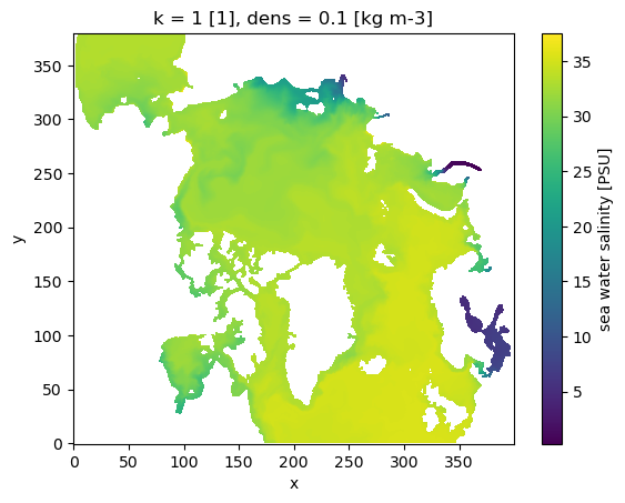
.compute() — return a new in-memory object, original stays lazy#
smean_lazy = ds_lazy['salin'].isel(k=0).mean('time')
smean_lazy
<xarray.DataArray 'salin' (y: 380, x: 400)> Size: 1MB
dask.array<mean_agg-aggregate, shape=(380, 400), dtype=float64, chunksize=(380, 400), chunktype=numpy.ndarray>
Coordinates:
    lon      (y, x) float64 1MB -94.75 -94.58 -94.42 ... 99.09 98.95 98.82
    lat      (y, x) float64 1MB 39.06 39.16 39.26 39.36 ... 56.39 56.29 56.2
    lon_u    (y, x) float64 1MB -94.83 -94.67 -94.5 -94.33 ... 99.16 99.02 98.89
    lat_u    (y, x) float64 1MB 39.01 39.11 39.21 39.31 ... 56.43 56.34 56.25
    lon_v    (y, x) float64 1MB -94.68 -94.52 -94.35 -94.19 ... 99.0 98.87 98.74
    lat_v    (y, x) float64 1MB 38.99 39.09 39.19 39.29 ... 56.43 56.33 56.24
    k        int64 8B 1
    dens     float64 8B dask.array<chunksize=(), meta=np.ndarray>
Dimensions without coordinates: y, x
Attributes:
    long_name:  sea water salinity
units: PSU- y: 380
- x: 400
- dask.array<chunksize=(380, 400), meta=np.ndarray>
Array Chunk Bytes 1.16 MiB 1.16 MiB Shape (380, 400) (380, 400) Dask graph 1 chunks in 23 graph layers Data type float64 numpy.ndarray - lon(y, x)float64-94.75 -94.58 ... 98.95 98.82
- long_name :
- longitude (T-point)
- units :
- degrees_east
- standard_name :
- longitude
array([[ -94.74750519, -94.58249664, -94.41687775, ..., 5.86695623, 6.06488323, 6.26205826], [ -94.87778473, -94.71282959, -94.5472641 , ..., 5.99605846, 6.1941061 , 6.391397 ], [ -95.00868225, -94.84378815, -94.67826843, ..., 6.12591982, 6.32408571, 6.5214901 ], ..., [-173.207901 , -173.30162048, -173.39605713, ..., 98.75035858, 98.61607361, 98.48277283], [-173.36988831, -173.46382141, -173.55848694, ..., 98.92017365, 98.78582764, 98.65245819], [-173.53115845, -173.62532043, -173.72019958, ..., 99.08900452, 98.95459747, 98.82115936]], shape=(380, 400)) - lat(y, x)float6439.06 39.16 39.26 ... 56.29 56.2
- long_name :
- latitude (T-point)
- units :
- degrees_north
- standard_name :
- latitude
array([[39.05597305, 39.15685272, 39.25762558, ..., 43.83851242, 43.74554825, 43.65235138], [39.18373108, 39.28490067, 39.38597107, ..., 43.98142242, 43.888134 , 43.79462051], [39.31121063, 39.41267776, 39.51403809, ..., 44.12407684, 44.03046799, 43.93662643], ..., [51.74200058, 51.84247589, 51.94287109, ..., 56.53710175, 56.44309616, 56.34889603], [51.68408203, 51.78424835, 51.88433075, ..., 56.46269226, 56.36904907, 56.27520752], [51.62594986, 51.72580338, 51.82557678, ..., 56.3881073 , 56.29482269, 56.20133972]], shape=(380, 400)) - lon_u(y, x)float64-94.83 -94.67 -94.5 ... 99.02 98.89
- long_name :
- longitude (U-point)
- units :
- degrees_east
array([[ -94.82977295, -94.66507721, -94.49976349, ..., 5.76771021, 5.96601391, 6.16356468], [ -94.9600296 , -94.79538727, -94.63012695, ..., 5.89674997, 6.09517717, 6.2928462 ], [ -95.09089661, -94.92630768, -94.7611084 , ..., 6.02655029, 6.22509813, 6.42288303], ..., [-173.16131592, -173.25466919, -173.34875488, ..., 98.81787109, 98.68309021, 98.54930115], [-173.32318115, -173.41676331, -173.51106262, ..., 98.98771667, 98.85287476, 98.71901703], [-173.48432922, -173.57815552, -173.67266846, ..., 99.15657806, 99.02167511, 98.88775635]], shape=(380, 400)) - lat_u(y, x)float6439.01 39.11 39.21 ... 56.34 56.25
- long_name :
- latitude (U-point)
- units :
- degrees_north
array([[39.00549698, 39.10642624, 39.2072525 , ..., 43.88490677, 43.79206085, 43.69897842], [39.13310623, 39.23432922, 39.33544922, ..., 44.02797699, 43.93480682, 43.84140778], [39.26044464, 39.36195755, 39.46337128, ..., 44.17079163, 44.07730103, 43.98357391], ..., [51.69173431, 51.79224777, 51.89268494, ..., 56.58403015, 56.49012375, 56.39601898], [51.63396835, 51.73417664, 51.83430099, ..., 56.50944138, 56.41589737, 56.32215118], [51.57598877, 51.67588806, 51.77569962, ..., 56.43467712, 56.3414917 , 56.24810791]], shape=(380, 400)) - lon_v(y, x)float64-94.68 -94.52 ... 98.87 98.74
- long_name :
- longitude (V-point)
- units :
- degrees_east
array([[ -94.6825943 , -94.51755524, -94.35191345, ..., 5.8026886 , 6.00055408, 6.19766998], [ -94.81256866, -94.64758301, -94.481987 , ..., 5.9314127 , 6.12940025, 6.32663393], [ -94.94315338, -94.77822876, -94.61268616, ..., 6.06089401, 6.25900126, 6.4563489 ], ..., [-173.12664795, -173.22024536, -173.3145752 , ..., 98.66507721, 98.53083038, 98.39756775], [-173.28898621, -173.3828125 , -173.47735596, ..., 98.83538818, 98.70107269, 98.56773376], [-173.4506073 , -173.54466248, -173.63943481, ..., 99.00471497, 98.87033081, 98.73693085]], shape=(380, 400)) - lat_v(y, x)float6438.99 39.09 39.19 ... 56.33 56.24
- long_name :
- latitude (V-point)
- units :
- degrees_north
array([[38.99199295, 39.09272385, 39.19335175, ..., 43.76696396, 43.67416 , 43.58112335], [39.11988831, 39.22091293, 39.32183075, ..., 43.90999985, 43.81687546, 43.72351837], [39.24750519, 39.34882355, 39.45003891, ..., 44.05278015, 43.95933151, 43.86565399], ..., [51.77088165, 51.87150955, 51.97205734, ..., 56.57423782, 56.48004913, 56.38566971], [51.71306992, 51.81338882, 51.91362762, ..., 56.49991989, 56.4060936 , 56.31207275], [51.65504074, 51.75505447, 51.85498047, ..., 56.42542267, 56.33195877, 56.23829651]], shape=(380, 400)) - k()int641
- long_name :
- layer index
- units :
- 1
- axis :
- Z
array(1)
- dens()float64dask.array<chunksize=(), meta=np.ndarray>
- long_name :
- target sigma-2 layer density
- units :
- kg m-3
Array Chunk Bytes 8 B 8 B Shape () () Dask graph 1 chunks in 2 graph layers Data type float64 numpy.ndarray
- long_name :
- sea water salinity
- units :
- PSU
smean = smean_lazy.compute() # smean_lazy is still a Dask array
smean_lazy
<xarray.DataArray 'salin' (y: 380, x: 400)> Size: 1MB
dask.array<mean_agg-aggregate, shape=(380, 400), dtype=float64, chunksize=(380, 400), chunktype=numpy.ndarray>
Coordinates:
    lon      (y, x) float64 1MB -94.75 -94.58 -94.42 ... 99.09 98.95 98.82
    lat      (y, x) float64 1MB 39.06 39.16 39.26 39.36 ... 56.39 56.29 56.2
    lon_u    (y, x) float64 1MB -94.83 -94.67 -94.5 -94.33 ... 99.16 99.02 98.89
    lat_u    (y, x) float64 1MB 39.01 39.11 39.21 39.31 ... 56.43 56.34 56.25
    lon_v    (y, x) float64 1MB -94.68 -94.52 -94.35 -94.19 ... 99.0 98.87 98.74
    lat_v    (y, x) float64 1MB 38.99 39.09 39.19 39.29 ... 56.43 56.33 56.24
    k        int64 8B 1
    dens     float64 8B dask.array<chunksize=(), meta=np.ndarray>
Dimensions without coordinates: y, x
Attributes:
    long_name:  sea water salinity
units: PSU- y: 380
- x: 400
- dask.array<chunksize=(380, 400), meta=np.ndarray>
Array Chunk Bytes 1.16 MiB 1.16 MiB Shape (380, 400) (380, 400) Dask graph 1 chunks in 23 graph layers Data type float64 numpy.ndarray - lon(y, x)float64-94.75 -94.58 ... 98.95 98.82
- long_name :
- longitude (T-point)
- units :
- degrees_east
- standard_name :
- longitude
array([[ -94.74750519, -94.58249664, -94.41687775, ..., 5.86695623, 6.06488323, 6.26205826], [ -94.87778473, -94.71282959, -94.5472641 , ..., 5.99605846, 6.1941061 , 6.391397 ], [ -95.00868225, -94.84378815, -94.67826843, ..., 6.12591982, 6.32408571, 6.5214901 ], ..., [-173.207901 , -173.30162048, -173.39605713, ..., 98.75035858, 98.61607361, 98.48277283], [-173.36988831, -173.46382141, -173.55848694, ..., 98.92017365, 98.78582764, 98.65245819], [-173.53115845, -173.62532043, -173.72019958, ..., 99.08900452, 98.95459747, 98.82115936]], shape=(380, 400)) - lat(y, x)float6439.06 39.16 39.26 ... 56.29 56.2
- long_name :
- latitude (T-point)
- units :
- degrees_north
- standard_name :
- latitude
array([[39.05597305, 39.15685272, 39.25762558, ..., 43.83851242, 43.74554825, 43.65235138], [39.18373108, 39.28490067, 39.38597107, ..., 43.98142242, 43.888134 , 43.79462051], [39.31121063, 39.41267776, 39.51403809, ..., 44.12407684, 44.03046799, 43.93662643], ..., [51.74200058, 51.84247589, 51.94287109, ..., 56.53710175, 56.44309616, 56.34889603], [51.68408203, 51.78424835, 51.88433075, ..., 56.46269226, 56.36904907, 56.27520752], [51.62594986, 51.72580338, 51.82557678, ..., 56.3881073 , 56.29482269, 56.20133972]], shape=(380, 400)) - lon_u(y, x)float64-94.83 -94.67 -94.5 ... 99.02 98.89
- long_name :
- longitude (U-point)
- units :
- degrees_east
array([[ -94.82977295, -94.66507721, -94.49976349, ..., 5.76771021, 5.96601391, 6.16356468], [ -94.9600296 , -94.79538727, -94.63012695, ..., 5.89674997, 6.09517717, 6.2928462 ], [ -95.09089661, -94.92630768, -94.7611084 , ..., 6.02655029, 6.22509813, 6.42288303], ..., [-173.16131592, -173.25466919, -173.34875488, ..., 98.81787109, 98.68309021, 98.54930115], [-173.32318115, -173.41676331, -173.51106262, ..., 98.98771667, 98.85287476, 98.71901703], [-173.48432922, -173.57815552, -173.67266846, ..., 99.15657806, 99.02167511, 98.88775635]], shape=(380, 400)) - lat_u(y, x)float6439.01 39.11 39.21 ... 56.34 56.25
- long_name :
- latitude (U-point)
- units :
- degrees_north
array([[39.00549698, 39.10642624, 39.2072525 , ..., 43.88490677, 43.79206085, 43.69897842], [39.13310623, 39.23432922, 39.33544922, ..., 44.02797699, 43.93480682, 43.84140778], [39.26044464, 39.36195755, 39.46337128, ..., 44.17079163, 44.07730103, 43.98357391], ..., [51.69173431, 51.79224777, 51.89268494, ..., 56.58403015, 56.49012375, 56.39601898], [51.63396835, 51.73417664, 51.83430099, ..., 56.50944138, 56.41589737, 56.32215118], [51.57598877, 51.67588806, 51.77569962, ..., 56.43467712, 56.3414917 , 56.24810791]], shape=(380, 400)) - lon_v(y, x)float64-94.68 -94.52 ... 98.87 98.74
- long_name :
- longitude (V-point)
- units :
- degrees_east
array([[ -94.6825943 , -94.51755524, -94.35191345, ..., 5.8026886 , 6.00055408, 6.19766998], [ -94.81256866, -94.64758301, -94.481987 , ..., 5.9314127 , 6.12940025, 6.32663393], [ -94.94315338, -94.77822876, -94.61268616, ..., 6.06089401, 6.25900126, 6.4563489 ], ..., [-173.12664795, -173.22024536, -173.3145752 , ..., 98.66507721, 98.53083038, 98.39756775], [-173.28898621, -173.3828125 , -173.47735596, ..., 98.83538818, 98.70107269, 98.56773376], [-173.4506073 , -173.54466248, -173.63943481, ..., 99.00471497, 98.87033081, 98.73693085]], shape=(380, 400)) - lat_v(y, x)float6438.99 39.09 39.19 ... 56.33 56.24
- long_name :
- latitude (V-point)
- units :
- degrees_north
array([[38.99199295, 39.09272385, 39.19335175, ..., 43.76696396, 43.67416 , 43.58112335], [39.11988831, 39.22091293, 39.32183075, ..., 43.90999985, 43.81687546, 43.72351837], [39.24750519, 39.34882355, 39.45003891, ..., 44.05278015, 43.95933151, 43.86565399], ..., [51.77088165, 51.87150955, 51.97205734, ..., 56.57423782, 56.48004913, 56.38566971], [51.71306992, 51.81338882, 51.91362762, ..., 56.49991989, 56.4060936 , 56.31207275], [51.65504074, 51.75505447, 51.85498047, ..., 56.42542267, 56.33195877, 56.23829651]], shape=(380, 400)) - k()int641
- long_name :
- layer index
- units :
- 1
- axis :
- Z
array(1)
- dens()float64dask.array<chunksize=(), meta=np.ndarray>
- long_name :
- target sigma-2 layer density
- units :
- kg m-3
Array Chunk Bytes 8 B 8 B Shape () () Dask graph 1 chunks in 2 graph layers Data type float64 numpy.ndarray
- long_name :
- sea water salinity
- units :
- PSU
smean
<xarray.DataArray 'salin' (y: 380, x: 400)> Size: 1MB
array([[nan, nan, nan, ..., nan, nan, nan],
       [nan, nan, nan, ..., nan, nan, nan],
       [nan, nan, nan, ..., nan, nan, nan],
       ...,
       [nan, nan, nan, ..., nan, nan, nan],
       [nan, nan, nan, ..., nan, nan, nan],
       [nan, nan, nan, ..., nan, nan, nan]], shape=(380, 400))
Coordinates:
    lon      (y, x) float64 1MB -94.75 -94.58 -94.42 ... 99.09 98.95 98.82
    lat      (y, x) float64 1MB 39.06 39.16 39.26 39.36 ... 56.39 56.29 56.2
    lon_u    (y, x) float64 1MB -94.83 -94.67 -94.5 -94.33 ... 99.16 99.02 98.89
    lat_u    (y, x) float64 1MB 39.01 39.11 39.21 39.31 ... 56.43 56.34 56.25
    lon_v    (y, x) float64 1MB -94.68 -94.52 -94.35 -94.19 ... 99.0 98.87 98.74
    lat_v    (y, x) float64 1MB 38.99 39.09 39.19 39.29 ... 56.43 56.33 56.24
    k        int64 8B 1
    dens     float64 8B 0.1
Dimensions without coordinates: y, x
Attributes:
    long_name:  sea water salinity
units: PSU- y: 380
- x: 400
- nan nan nan nan nan nan nan nan ... nan nan nan nan nan nan nan nan
array([[nan, nan, nan, ..., nan, nan, nan], [nan, nan, nan, ..., nan, nan, nan], [nan, nan, nan, ..., nan, nan, nan], ..., [nan, nan, nan, ..., nan, nan, nan], [nan, nan, nan, ..., nan, nan, nan], [nan, nan, nan, ..., nan, nan, nan]], shape=(380, 400)) - lon(y, x)float64-94.75 -94.58 ... 98.95 98.82
- long_name :
- longitude (T-point)
- units :
- degrees_east
- standard_name :
- longitude
array([[ -94.74750519, -94.58249664, -94.41687775, ..., 5.86695623, 6.06488323, 6.26205826], [ -94.87778473, -94.71282959, -94.5472641 , ..., 5.99605846, 6.1941061 , 6.391397 ], [ -95.00868225, -94.84378815, -94.67826843, ..., 6.12591982, 6.32408571, 6.5214901 ], ..., [-173.207901 , -173.30162048, -173.39605713, ..., 98.75035858, 98.61607361, 98.48277283], [-173.36988831, -173.46382141, -173.55848694, ..., 98.92017365, 98.78582764, 98.65245819], [-173.53115845, -173.62532043, -173.72019958, ..., 99.08900452, 98.95459747, 98.82115936]], shape=(380, 400)) - lat(y, x)float6439.06 39.16 39.26 ... 56.29 56.2
- long_name :
- latitude (T-point)
- units :
- degrees_north
- standard_name :
- latitude
array([[39.05597305, 39.15685272, 39.25762558, ..., 43.83851242, 43.74554825, 43.65235138], [39.18373108, 39.28490067, 39.38597107, ..., 43.98142242, 43.888134 , 43.79462051], [39.31121063, 39.41267776, 39.51403809, ..., 44.12407684, 44.03046799, 43.93662643], ..., [51.74200058, 51.84247589, 51.94287109, ..., 56.53710175, 56.44309616, 56.34889603], [51.68408203, 51.78424835, 51.88433075, ..., 56.46269226, 56.36904907, 56.27520752], [51.62594986, 51.72580338, 51.82557678, ..., 56.3881073 , 56.29482269, 56.20133972]], shape=(380, 400)) - lon_u(y, x)float64-94.83 -94.67 -94.5 ... 99.02 98.89
- long_name :
- longitude (U-point)
- units :
- degrees_east
array([[ -94.82977295, -94.66507721, -94.49976349, ..., 5.76771021, 5.96601391, 6.16356468], [ -94.9600296 , -94.79538727, -94.63012695, ..., 5.89674997, 6.09517717, 6.2928462 ], [ -95.09089661, -94.92630768, -94.7611084 , ..., 6.02655029, 6.22509813, 6.42288303], ..., [-173.16131592, -173.25466919, -173.34875488, ..., 98.81787109, 98.68309021, 98.54930115], [-173.32318115, -173.41676331, -173.51106262, ..., 98.98771667, 98.85287476, 98.71901703], [-173.48432922, -173.57815552, -173.67266846, ..., 99.15657806, 99.02167511, 98.88775635]], shape=(380, 400)) - lat_u(y, x)float6439.01 39.11 39.21 ... 56.34 56.25
- long_name :
- latitude (U-point)
- units :
- degrees_north
array([[39.00549698, 39.10642624, 39.2072525 , ..., 43.88490677, 43.79206085, 43.69897842], [39.13310623, 39.23432922, 39.33544922, ..., 44.02797699, 43.93480682, 43.84140778], [39.26044464, 39.36195755, 39.46337128, ..., 44.17079163, 44.07730103, 43.98357391], ..., [51.69173431, 51.79224777, 51.89268494, ..., 56.58403015, 56.49012375, 56.39601898], [51.63396835, 51.73417664, 51.83430099, ..., 56.50944138, 56.41589737, 56.32215118], [51.57598877, 51.67588806, 51.77569962, ..., 56.43467712, 56.3414917 , 56.24810791]], shape=(380, 400)) - lon_v(y, x)float64-94.68 -94.52 ... 98.87 98.74
- long_name :
- longitude (V-point)
- units :
- degrees_east
array([[ -94.6825943 , -94.51755524, -94.35191345, ..., 5.8026886 , 6.00055408, 6.19766998], [ -94.81256866, -94.64758301, -94.481987 , ..., 5.9314127 , 6.12940025, 6.32663393], [ -94.94315338, -94.77822876, -94.61268616, ..., 6.06089401, 6.25900126, 6.4563489 ], ..., [-173.12664795, -173.22024536, -173.3145752 , ..., 98.66507721, 98.53083038, 98.39756775], [-173.28898621, -173.3828125 , -173.47735596, ..., 98.83538818, 98.70107269, 98.56773376], [-173.4506073 , -173.54466248, -173.63943481, ..., 99.00471497, 98.87033081, 98.73693085]], shape=(380, 400)) - lat_v(y, x)float6438.99 39.09 39.19 ... 56.33 56.24
- long_name :
- latitude (V-point)
- units :
- degrees_north
array([[38.99199295, 39.09272385, 39.19335175, ..., 43.76696396, 43.67416 , 43.58112335], [39.11988831, 39.22091293, 39.32183075, ..., 43.90999985, 43.81687546, 43.72351837], [39.24750519, 39.34882355, 39.45003891, ..., 44.05278015, 43.95933151, 43.86565399], ..., [51.77088165, 51.87150955, 51.97205734, ..., 56.57423782, 56.48004913, 56.38566971], [51.71306992, 51.81338882, 51.91362762, ..., 56.49991989, 56.4060936 , 56.31207275], [51.65504074, 51.75505447, 51.85498047, ..., 56.42542267, 56.33195877, 56.23829651]], shape=(380, 400)) - k()int641
- long_name :
- layer index
- units :
- 1
- axis :
- Z
array(1)
- dens()float640.1
- long_name :
- target sigma-2 layer density
- units :
- kg m-3
array(0.1)
- long_name :
- sea water salinity
- units :
- PSU
smean.plot() # fast
<matplotlib.collections.QuadMesh at 0x153caa633e50>
.plot() — compute on the fly, result not stored#
Use .plot() for quick inspection. If you need the values afterwards, call .load() or .compute() first.
# .plot() computes internally — no need to load first
smean_lazy = ds_lazy['salin'].isel(k=0).mean('time')
smean_lazy.plot()   # reads from disk, plots, discards the computed values
<matplotlib.collections.QuadMesh at 0x153ca617bf90>
smean_lazy
<xarray.DataArray 'salin' (y: 380, x: 400)> Size: 1MB
dask.array<mean_agg-aggregate, shape=(380, 400), dtype=float64, chunksize=(380, 400), chunktype=numpy.ndarray>
Coordinates:
    lon      (y, x) float64 1MB -94.75 -94.58 -94.42 ... 99.09 98.95 98.82
    lat      (y, x) float64 1MB 39.06 39.16 39.26 39.36 ... 56.39 56.29 56.2
    lon_u    (y, x) float64 1MB -94.83 -94.67 -94.5 -94.33 ... 99.16 99.02 98.89
    lat_u    (y, x) float64 1MB 39.01 39.11 39.21 39.31 ... 56.43 56.34 56.25
    lon_v    (y, x) float64 1MB -94.68 -94.52 -94.35 -94.19 ... 99.0 98.87 98.74
    lat_v    (y, x) float64 1MB 38.99 39.09 39.19 39.29 ... 56.43 56.33 56.24
    k        int64 8B 1
    dens     float64 8B dask.array<chunksize=(), meta=np.ndarray>
Dimensions without coordinates: y, x
Attributes:
    long_name:  sea water salinity
units: PSU- y: 380
- x: 400
- dask.array<chunksize=(380, 400), meta=np.ndarray>
Array Chunk Bytes 1.16 MiB 1.16 MiB Shape (380, 400) (380, 400) Dask graph 1 chunks in 23 graph layers Data type float64 numpy.ndarray - lon(y, x)float64-94.75 -94.58 ... 98.95 98.82
- long_name :
- longitude (T-point)
- units :
- degrees_east
- standard_name :
- longitude
array([[ -94.74750519, -94.58249664, -94.41687775, ..., 5.86695623, 6.06488323, 6.26205826], [ -94.87778473, -94.71282959, -94.5472641 , ..., 5.99605846, 6.1941061 , 6.391397 ], [ -95.00868225, -94.84378815, -94.67826843, ..., 6.12591982, 6.32408571, 6.5214901 ], ..., [-173.207901 , -173.30162048, -173.39605713, ..., 98.75035858, 98.61607361, 98.48277283], [-173.36988831, -173.46382141, -173.55848694, ..., 98.92017365, 98.78582764, 98.65245819], [-173.53115845, -173.62532043, -173.72019958, ..., 99.08900452, 98.95459747, 98.82115936]], shape=(380, 400)) - lat(y, x)float6439.06 39.16 39.26 ... 56.29 56.2
- long_name :
- latitude (T-point)
- units :
- degrees_north
- standard_name :
- latitude
array([[39.05597305, 39.15685272, 39.25762558, ..., 43.83851242, 43.74554825, 43.65235138], [39.18373108, 39.28490067, 39.38597107, ..., 43.98142242, 43.888134 , 43.79462051], [39.31121063, 39.41267776, 39.51403809, ..., 44.12407684, 44.03046799, 43.93662643], ..., [51.74200058, 51.84247589, 51.94287109, ..., 56.53710175, 56.44309616, 56.34889603], [51.68408203, 51.78424835, 51.88433075, ..., 56.46269226, 56.36904907, 56.27520752], [51.62594986, 51.72580338, 51.82557678, ..., 56.3881073 , 56.29482269, 56.20133972]], shape=(380, 400)) - lon_u(y, x)float64-94.83 -94.67 -94.5 ... 99.02 98.89
- long_name :
- longitude (U-point)
- units :
- degrees_east
array([[ -94.82977295, -94.66507721, -94.49976349, ..., 5.76771021, 5.96601391, 6.16356468], [ -94.9600296 , -94.79538727, -94.63012695, ..., 5.89674997, 6.09517717, 6.2928462 ], [ -95.09089661, -94.92630768, -94.7611084 , ..., 6.02655029, 6.22509813, 6.42288303], ..., [-173.16131592, -173.25466919, -173.34875488, ..., 98.81787109, 98.68309021, 98.54930115], [-173.32318115, -173.41676331, -173.51106262, ..., 98.98771667, 98.85287476, 98.71901703], [-173.48432922, -173.57815552, -173.67266846, ..., 99.15657806, 99.02167511, 98.88775635]], shape=(380, 400)) - lat_u(y, x)float6439.01 39.11 39.21 ... 56.34 56.25
- long_name :
- latitude (U-point)
- units :
- degrees_north
array([[39.00549698, 39.10642624, 39.2072525 , ..., 43.88490677, 43.79206085, 43.69897842], [39.13310623, 39.23432922, 39.33544922, ..., 44.02797699, 43.93480682, 43.84140778], [39.26044464, 39.36195755, 39.46337128, ..., 44.17079163, 44.07730103, 43.98357391], ..., [51.69173431, 51.79224777, 51.89268494, ..., 56.58403015, 56.49012375, 56.39601898], [51.63396835, 51.73417664, 51.83430099, ..., 56.50944138, 56.41589737, 56.32215118], [51.57598877, 51.67588806, 51.77569962, ..., 56.43467712, 56.3414917 , 56.24810791]], shape=(380, 400)) - lon_v(y, x)float64-94.68 -94.52 ... 98.87 98.74
- long_name :
- longitude (V-point)
- units :
- degrees_east
array([[ -94.6825943 , -94.51755524, -94.35191345, ..., 5.8026886 , 6.00055408, 6.19766998], [ -94.81256866, -94.64758301, -94.481987 , ..., 5.9314127 , 6.12940025, 6.32663393], [ -94.94315338, -94.77822876, -94.61268616, ..., 6.06089401, 6.25900126, 6.4563489 ], ..., [-173.12664795, -173.22024536, -173.3145752 , ..., 98.66507721, 98.53083038, 98.39756775], [-173.28898621, -173.3828125 , -173.47735596, ..., 98.83538818, 98.70107269, 98.56773376], [-173.4506073 , -173.54466248, -173.63943481, ..., 99.00471497, 98.87033081, 98.73693085]], shape=(380, 400)) - lat_v(y, x)float6438.99 39.09 39.19 ... 56.33 56.24
- long_name :
- latitude (V-point)
- units :
- degrees_north
array([[38.99199295, 39.09272385, 39.19335175, ..., 43.76696396, 43.67416 , 43.58112335], [39.11988831, 39.22091293, 39.32183075, ..., 43.90999985, 43.81687546, 43.72351837], [39.24750519, 39.34882355, 39.45003891, ..., 44.05278015, 43.95933151, 43.86565399], ..., [51.77088165, 51.87150955, 51.97205734, ..., 56.57423782, 56.48004913, 56.38566971], [51.71306992, 51.81338882, 51.91362762, ..., 56.49991989, 56.4060936 , 56.31207275], [51.65504074, 51.75505447, 51.85498047, ..., 56.42542267, 56.33195877, 56.23829651]], shape=(380, 400)) - k()int641
- long_name :
- layer index
- units :
- 1
- axis :
- Z
array(1)
- dens()float64dask.array<chunksize=(), meta=np.ndarray>
- long_name :
- target sigma-2 layer density
- units :
- kg m-3
Array Chunk Bytes 8 B 8 B Shape () () Dask graph 1 chunks in 2 graph layers Data type float64 numpy.ndarray
- long_name :
- sea water salinity
- units :
- PSU
.to_netcdf() — compute and write to disk#
smean_lazy = ds_lazy['salin'].isel(k=0).mean('time')
smean_lazy.to_netcdf('smean_salin.nc')  # triggers full compute, writes result
smean_lazy
<xarray.DataArray 'salin' (y: 380, x: 400)> Size: 1MB
dask.array<mean_agg-aggregate, shape=(380, 400), dtype=float64, chunksize=(380, 400), chunktype=numpy.ndarray>
Coordinates:
    lon      (y, x) float64 1MB -94.75 -94.58 -94.42 ... 99.09 98.95 98.82
    lat      (y, x) float64 1MB 39.06 39.16 39.26 39.36 ... 56.39 56.29 56.2
    lon_u    (y, x) float64 1MB -94.83 -94.67 -94.5 -94.33 ... 99.16 99.02 98.89
    lat_u    (y, x) float64 1MB 39.01 39.11 39.21 39.31 ... 56.43 56.34 56.25
    lon_v    (y, x) float64 1MB -94.68 -94.52 -94.35 -94.19 ... 99.0 98.87 98.74
    lat_v    (y, x) float64 1MB 38.99 39.09 39.19 39.29 ... 56.43 56.33 56.24
    k        int64 8B 1
    dens     float64 8B dask.array<chunksize=(), meta=np.ndarray>
Dimensions without coordinates: y, x
Attributes:
    long_name:  sea water salinity
units: PSU- y: 380
- x: 400
- dask.array<chunksize=(380, 400), meta=np.ndarray>
Array Chunk Bytes 1.16 MiB 1.16 MiB Shape (380, 400) (380, 400) Dask graph 1 chunks in 23 graph layers Data type float64 numpy.ndarray - lon(y, x)float64-94.75 -94.58 ... 98.95 98.82
- long_name :
- longitude (T-point)
- units :
- degrees_east
- standard_name :
- longitude
array([[ -94.74750519, -94.58249664, -94.41687775, ..., 5.86695623, 6.06488323, 6.26205826], [ -94.87778473, -94.71282959, -94.5472641 , ..., 5.99605846, 6.1941061 , 6.391397 ], [ -95.00868225, -94.84378815, -94.67826843, ..., 6.12591982, 6.32408571, 6.5214901 ], ..., [-173.207901 , -173.30162048, -173.39605713, ..., 98.75035858, 98.61607361, 98.48277283], [-173.36988831, -173.46382141, -173.55848694, ..., 98.92017365, 98.78582764, 98.65245819], [-173.53115845, -173.62532043, -173.72019958, ..., 99.08900452, 98.95459747, 98.82115936]], shape=(380, 400)) - lat(y, x)float6439.06 39.16 39.26 ... 56.29 56.2
- long_name :
- latitude (T-point)
- units :
- degrees_north
- standard_name :
- latitude
array([[39.05597305, 39.15685272, 39.25762558, ..., 43.83851242, 43.74554825, 43.65235138], [39.18373108, 39.28490067, 39.38597107, ..., 43.98142242, 43.888134 , 43.79462051], [39.31121063, 39.41267776, 39.51403809, ..., 44.12407684, 44.03046799, 43.93662643], ..., [51.74200058, 51.84247589, 51.94287109, ..., 56.53710175, 56.44309616, 56.34889603], [51.68408203, 51.78424835, 51.88433075, ..., 56.46269226, 56.36904907, 56.27520752], [51.62594986, 51.72580338, 51.82557678, ..., 56.3881073 , 56.29482269, 56.20133972]], shape=(380, 400)) - lon_u(y, x)float64-94.83 -94.67 -94.5 ... 99.02 98.89
- long_name :
- longitude (U-point)
- units :
- degrees_east
array([[ -94.82977295, -94.66507721, -94.49976349, ..., 5.76771021, 5.96601391, 6.16356468], [ -94.9600296 , -94.79538727, -94.63012695, ..., 5.89674997, 6.09517717, 6.2928462 ], [ -95.09089661, -94.92630768, -94.7611084 , ..., 6.02655029, 6.22509813, 6.42288303], ..., [-173.16131592, -173.25466919, -173.34875488, ..., 98.81787109, 98.68309021, 98.54930115], [-173.32318115, -173.41676331, -173.51106262, ..., 98.98771667, 98.85287476, 98.71901703], [-173.48432922, -173.57815552, -173.67266846, ..., 99.15657806, 99.02167511, 98.88775635]], shape=(380, 400)) - lat_u(y, x)float6439.01 39.11 39.21 ... 56.34 56.25
- long_name :
- latitude (U-point)
- units :
- degrees_north
array([[39.00549698, 39.10642624, 39.2072525 , ..., 43.88490677, 43.79206085, 43.69897842], [39.13310623, 39.23432922, 39.33544922, ..., 44.02797699, 43.93480682, 43.84140778], [39.26044464, 39.36195755, 39.46337128, ..., 44.17079163, 44.07730103, 43.98357391], ..., [51.69173431, 51.79224777, 51.89268494, ..., 56.58403015, 56.49012375, 56.39601898], [51.63396835, 51.73417664, 51.83430099, ..., 56.50944138, 56.41589737, 56.32215118], [51.57598877, 51.67588806, 51.77569962, ..., 56.43467712, 56.3414917 , 56.24810791]], shape=(380, 400)) - lon_v(y, x)float64-94.68 -94.52 ... 98.87 98.74
- long_name :
- longitude (V-point)
- units :
- degrees_east
array([[ -94.6825943 , -94.51755524, -94.35191345, ..., 5.8026886 , 6.00055408, 6.19766998], [ -94.81256866, -94.64758301, -94.481987 , ..., 5.9314127 , 6.12940025, 6.32663393], [ -94.94315338, -94.77822876, -94.61268616, ..., 6.06089401, 6.25900126, 6.4563489 ], ..., [-173.12664795, -173.22024536, -173.3145752 , ..., 98.66507721, 98.53083038, 98.39756775], [-173.28898621, -173.3828125 , -173.47735596, ..., 98.83538818, 98.70107269, 98.56773376], [-173.4506073 , -173.54466248, -173.63943481, ..., 99.00471497, 98.87033081, 98.73693085]], shape=(380, 400)) - lat_v(y, x)float6438.99 39.09 39.19 ... 56.33 56.24
- long_name :
- latitude (V-point)
- units :
- degrees_north
array([[38.99199295, 39.09272385, 39.19335175, ..., 43.76696396, 43.67416 , 43.58112335], [39.11988831, 39.22091293, 39.32183075, ..., 43.90999985, 43.81687546, 43.72351837], [39.24750519, 39.34882355, 39.45003891, ..., 44.05278015, 43.95933151, 43.86565399], ..., [51.77088165, 51.87150955, 51.97205734, ..., 56.57423782, 56.48004913, 56.38566971], [51.71306992, 51.81338882, 51.91362762, ..., 56.49991989, 56.4060936 , 56.31207275], [51.65504074, 51.75505447, 51.85498047, ..., 56.42542267, 56.33195877, 56.23829651]], shape=(380, 400)) - k()int641
- long_name :
- layer index
- units :
- 1
- axis :
- Z
array(1)
- dens()float64dask.array<chunksize=(), meta=np.ndarray>
- long_name :
- target sigma-2 layer density
- units :
- kg m-3
Array Chunk Bytes 8 B 8 B Shape () () Dask graph 1 chunks in 2 graph layers Data type float64 numpy.ndarray
- long_name :
- sea water salinity
- units :
- PSU
.values — compute and return a NumPy array#
smean_lazy = ds_lazy['salin'].isel(k=0).mean('time')
arr = smean_lazy.values   # plain NumPy array, e.g. for scipy / sklearn
smean_lazy
<xarray.DataArray 'salin' (y: 380, x: 400)> Size: 1MB
dask.array<mean_agg-aggregate, shape=(380, 400), dtype=float64, chunksize=(380, 400), chunktype=numpy.ndarray>
Coordinates:
    lon      (y, x) float64 1MB -94.75 -94.58 -94.42 ... 99.09 98.95 98.82
    lat      (y, x) float64 1MB 39.06 39.16 39.26 39.36 ... 56.39 56.29 56.2
    lon_u    (y, x) float64 1MB -94.83 -94.67 -94.5 -94.33 ... 99.16 99.02 98.89
    lat_u    (y, x) float64 1MB 39.01 39.11 39.21 39.31 ... 56.43 56.34 56.25
    lon_v    (y, x) float64 1MB -94.68 -94.52 -94.35 -94.19 ... 99.0 98.87 98.74
    lat_v    (y, x) float64 1MB 38.99 39.09 39.19 39.29 ... 56.43 56.33 56.24
    k        int64 8B 1
    dens     float64 8B dask.array<chunksize=(), meta=np.ndarray>
Dimensions without coordinates: y, x
Attributes:
    long_name:  sea water salinity
units: PSU- y: 380
- x: 400
- dask.array<chunksize=(380, 400), meta=np.ndarray>
Array Chunk Bytes 1.16 MiB 1.16 MiB Shape (380, 400) (380, 400) Dask graph 1 chunks in 23 graph layers Data type float64 numpy.ndarray - lon(y, x)float64-94.75 -94.58 ... 98.95 98.82
- long_name :
- longitude (T-point)
- units :
- degrees_east
- standard_name :
- longitude
array([[ -94.74750519, -94.58249664, -94.41687775, ..., 5.86695623, 6.06488323, 6.26205826], [ -94.87778473, -94.71282959, -94.5472641 , ..., 5.99605846, 6.1941061 , 6.391397 ], [ -95.00868225, -94.84378815, -94.67826843, ..., 6.12591982, 6.32408571, 6.5214901 ], ..., [-173.207901 , -173.30162048, -173.39605713, ..., 98.75035858, 98.61607361, 98.48277283], [-173.36988831, -173.46382141, -173.55848694, ..., 98.92017365, 98.78582764, 98.65245819], [-173.53115845, -173.62532043, -173.72019958, ..., 99.08900452, 98.95459747, 98.82115936]], shape=(380, 400)) - lat(y, x)float6439.06 39.16 39.26 ... 56.29 56.2
- long_name :
- latitude (T-point)
- units :
- degrees_north
- standard_name :
- latitude
array([[39.05597305, 39.15685272, 39.25762558, ..., 43.83851242, 43.74554825, 43.65235138], [39.18373108, 39.28490067, 39.38597107, ..., 43.98142242, 43.888134 , 43.79462051], [39.31121063, 39.41267776, 39.51403809, ..., 44.12407684, 44.03046799, 43.93662643], ..., [51.74200058, 51.84247589, 51.94287109, ..., 56.53710175, 56.44309616, 56.34889603], [51.68408203, 51.78424835, 51.88433075, ..., 56.46269226, 56.36904907, 56.27520752], [51.62594986, 51.72580338, 51.82557678, ..., 56.3881073 , 56.29482269, 56.20133972]], shape=(380, 400)) - lon_u(y, x)float64-94.83 -94.67 -94.5 ... 99.02 98.89
- long_name :
- longitude (U-point)
- units :
- degrees_east
array([[ -94.82977295, -94.66507721, -94.49976349, ..., 5.76771021, 5.96601391, 6.16356468], [ -94.9600296 , -94.79538727, -94.63012695, ..., 5.89674997, 6.09517717, 6.2928462 ], [ -95.09089661, -94.92630768, -94.7611084 , ..., 6.02655029, 6.22509813, 6.42288303], ..., [-173.16131592, -173.25466919, -173.34875488, ..., 98.81787109, 98.68309021, 98.54930115], [-173.32318115, -173.41676331, -173.51106262, ..., 98.98771667, 98.85287476, 98.71901703], [-173.48432922, -173.57815552, -173.67266846, ..., 99.15657806, 99.02167511, 98.88775635]], shape=(380, 400)) - lat_u(y, x)float6439.01 39.11 39.21 ... 56.34 56.25
- long_name :
- latitude (U-point)
- units :
- degrees_north
array([[39.00549698, 39.10642624, 39.2072525 , ..., 43.88490677, 43.79206085, 43.69897842], [39.13310623, 39.23432922, 39.33544922, ..., 44.02797699, 43.93480682, 43.84140778], [39.26044464, 39.36195755, 39.46337128, ..., 44.17079163, 44.07730103, 43.98357391], ..., [51.69173431, 51.79224777, 51.89268494, ..., 56.58403015, 56.49012375, 56.39601898], [51.63396835, 51.73417664, 51.83430099, ..., 56.50944138, 56.41589737, 56.32215118], [51.57598877, 51.67588806, 51.77569962, ..., 56.43467712, 56.3414917 , 56.24810791]], shape=(380, 400)) - lon_v(y, x)float64-94.68 -94.52 ... 98.87 98.74
- long_name :
- longitude (V-point)
- units :
- degrees_east
array([[ -94.6825943 , -94.51755524, -94.35191345, ..., 5.8026886 , 6.00055408, 6.19766998], [ -94.81256866, -94.64758301, -94.481987 , ..., 5.9314127 , 6.12940025, 6.32663393], [ -94.94315338, -94.77822876, -94.61268616, ..., 6.06089401, 6.25900126, 6.4563489 ], ..., [-173.12664795, -173.22024536, -173.3145752 , ..., 98.66507721, 98.53083038, 98.39756775], [-173.28898621, -173.3828125 , -173.47735596, ..., 98.83538818, 98.70107269, 98.56773376], [-173.4506073 , -173.54466248, -173.63943481, ..., 99.00471497, 98.87033081, 98.73693085]], shape=(380, 400)) - lat_v(y, x)float6438.99 39.09 39.19 ... 56.33 56.24
- long_name :
- latitude (V-point)
- units :
- degrees_north
array([[38.99199295, 39.09272385, 39.19335175, ..., 43.76696396, 43.67416 , 43.58112335], [39.11988831, 39.22091293, 39.32183075, ..., 43.90999985, 43.81687546, 43.72351837], [39.24750519, 39.34882355, 39.45003891, ..., 44.05278015, 43.95933151, 43.86565399], ..., [51.77088165, 51.87150955, 51.97205734, ..., 56.57423782, 56.48004913, 56.38566971], [51.71306992, 51.81338882, 51.91362762, ..., 56.49991989, 56.4060936 , 56.31207275], [51.65504074, 51.75505447, 51.85498047, ..., 56.42542267, 56.33195877, 56.23829651]], shape=(380, 400)) - k()int641
- long_name :
- layer index
- units :
- 1
- axis :
- Z
array(1)
- dens()float64dask.array<chunksize=(), meta=np.ndarray>
- long_name :
- target sigma-2 layer density
- units :
- kg m-3
Array Chunk Bytes 8 B 8 B Shape () () Dask graph 1 chunks in 2 graph layers Data type float64 numpy.ndarray
- long_name :
- sea water salinity
- units :
- PSU
Tip
Use .load() when you want to reuse a result multiple times — one disk read, then everything is fast. Use .compute() when you want to keep a lazy original and hand a concrete copy to other code.
Putting it together for long time series#
The same methods apply at any scale. Here we compute the spatial-mean sea-surface height across 30 years and save it directly to NetCDF — Dask streams through the 11 805 files one chunk at a time.
%%time
%%memit

ds_lazy = xhycom.open_mfdataset(DATA_PATH + "archm.2020*", grid=GRID_PATH, chunks={"time": 1})
peak memory: 28518.71 MiB, increment: 414.06 MiB
CPU times: user 8.98 s, sys: 184 ms, total: 9.17 s
Wall time: 9.24 s
ds_lazy
<xarray.Dataset> Size: 1TB
Dimensions:     (y: 380, x: 400, time: 366, k: 50, ki: 51)
Coordinates:
    lon         (y, x) float64 1MB dask.array<chunksize=(380, 400), meta=np.ndarray>
    lat         (y, x) float64 1MB dask.array<chunksize=(380, 400), meta=np.ndarray>
    lon_u       (y, x) float64 1MB dask.array<chunksize=(380, 400), meta=np.ndarray>
    lat_u       (y, x) float64 1MB dask.array<chunksize=(380, 400), meta=np.ndarray>
    lon_v       (y, x) float64 1MB dask.array<chunksize=(380, 400), meta=np.ndarray>
    lat_v       (y, x) float64 1MB dask.array<chunksize=(380, 400), meta=np.ndarray>
  * time        (time) object 3kB 2020-01-01 00:00:00 ... 2020-12-31 00:00:00
  * k           (k) int64 400B 1 2 3 4 5 6 7 8 9 ... 42 43 44 45 46 47 48 49 50
    dens        (k) float64 400B dask.array<chunksize=(50,), meta=np.ndarray>
  * ki          (ki) int64 408B 0 1 2 3 4 5 6 7 8 ... 42 43 44 45 46 47 48 49 50
Dimensions without coordinates: y, x
Data variables: (12/83)
    montg1      (time, y, x) float64 445MB dask.array<chunksize=(1, 380, 400), meta=np.ndarray>
    srfhgt      (time, y, x) float64 445MB dask.array<chunksize=(1, 380, 400), meta=np.ndarray>
    oneta       (time, y, x) float64 445MB dask.array<chunksize=(1, 380, 400), meta=np.ndarray>
    surflx      (time, y, x) float64 445MB dask.array<chunksize=(1, 380, 400), meta=np.ndarray>
    wtrflx      (time, y, x) float64 445MB dask.array<chunksize=(1, 380, 400), meta=np.ndarray>
    salflx      (time, y, x) float64 445MB dask.array<chunksize=(1, 380, 400), meta=np.ndarray>
    ...          ...
    CO2_wind    (time, y, x) float64 445MB dask.array<chunksize=(1, 380, 400), meta=np.ndarray>
    ECO_bots    (time, y, x) float64 445MB dask.array<chunksize=(1, 380, 400), meta=np.ndarray>
    surface__1  (time, y, x) float64 445MB dask.array<chunksize=(1, 380, 400), meta=np.ndarray>
    surface__2  (time, y, x) float64 445MB dask.array<chunksize=(1, 380, 400), meta=np.ndarray>
    si_u        (time, y, x) float64 445MB dask.array<chunksize=(1, 380, 400), meta=np.ndarray>
    si_v        (time, y, x) float64 445MB dask.array<chunksize=(1, 380, 400), meta=np.ndarray>
Attributes:
    iversn:   23
    iexpt:    28
yrflag: 3- y: 380
- x: 400
- time: 366
- k: 50
- ki: 51
- lon(y, x)float64dask.array<chunksize=(380, 400), meta=np.ndarray>
- long_name :
- longitude (T-point)
- units :
- degrees_east
- standard_name :
- longitude
Array Chunk Bytes 1.16 MiB 1.16 MiB Shape (380, 400) (380, 400) Dask graph 1 chunks in 1 graph layer Data type float64 numpy.ndarray - lat(y, x)float64dask.array<chunksize=(380, 400), meta=np.ndarray>
- long_name :
- latitude (T-point)
- units :
- degrees_north
- standard_name :
- latitude
Array Chunk Bytes 1.16 MiB 1.16 MiB Shape (380, 400) (380, 400) Dask graph 1 chunks in 1 graph layer Data type float64 numpy.ndarray - lon_u(y, x)float64dask.array<chunksize=(380, 400), meta=np.ndarray>
- long_name :
- longitude (U-point)
- units :
- degrees_east
Array Chunk Bytes 1.16 MiB 1.16 MiB Shape (380, 400) (380, 400) Dask graph 1 chunks in 1 graph layer Data type float64 numpy.ndarray - lat_u(y, x)float64dask.array<chunksize=(380, 400), meta=np.ndarray>
- long_name :
- latitude (U-point)
- units :
- degrees_north
Array Chunk Bytes 1.16 MiB 1.16 MiB Shape (380, 400) (380, 400) Dask graph 1 chunks in 1 graph layer Data type float64 numpy.ndarray - lon_v(y, x)float64dask.array<chunksize=(380, 400), meta=np.ndarray>
- long_name :
- longitude (V-point)
- units :
- degrees_east
Array Chunk Bytes 1.16 MiB 1.16 MiB Shape (380, 400) (380, 400) Dask graph 1 chunks in 1 graph layer Data type float64 numpy.ndarray - lat_v(y, x)float64dask.array<chunksize=(380, 400), meta=np.ndarray>
- long_name :
- latitude (V-point)
- units :
- degrees_north
Array Chunk Bytes 1.16 MiB 1.16 MiB Shape (380, 400) (380, 400) Dask graph 1 chunks in 1 graph layer Data type float64 numpy.ndarray - time(time)object2020-01-01 00:00:00 ... 2020-12-...
- long_name :
- time
- axis :
- T
array([cftime.DatetimeGregorian(2020, 1, 1, 0, 0, 0, 0, has_year_zero=False), cftime.DatetimeGregorian(2020, 1, 2, 0, 0, 0, 0, has_year_zero=False), cftime.DatetimeGregorian(2020, 1, 3, 0, 0, 0, 0, has_year_zero=False), ..., cftime.DatetimeGregorian(2020, 12, 29, 0, 0, 0, 0, has_year_zero=False), cftime.DatetimeGregorian(2020, 12, 30, 0, 0, 0, 0, has_year_zero=False), cftime.DatetimeGregorian(2020, 12, 31, 0, 0, 0, 0, has_year_zero=False)], shape=(366,), dtype=object) - k(k)int641 2 3 4 5 6 7 ... 45 46 47 48 49 50
- long_name :
- layer index
- units :
- 1
- axis :
- Z
array([ 1, 2, 3, 4, 5, 6, 7, 8, 9, 10, 11, 12, 13, 14, 15, 16, 17, 18, 19, 20, 21, 22, 23, 24, 25, 26, 27, 28, 29, 30, 31, 32, 33, 34, 35, 36, 37, 38, 39, 40, 41, 42, 43, 44, 45, 46, 47, 48, 49, 50]) - dens(k)float64dask.array<chunksize=(50,), meta=np.ndarray>
- long_name :
- target sigma-2 layer density
- units :
- kg m-3
Array Chunk Bytes 400 B 400 B Shape (50,) (50,) Dask graph 1 chunks in 1 graph layer Data type float64 numpy.ndarray - ki(ki)int640 1 2 3 4 5 6 ... 45 46 47 48 49 50
- long_name :
- layer interface index
- units :
- 1
- axis :
- Z
array([ 0,  1,  2,  3,  4,  5,  6,  7,  8,  9, 10, 11, 12, 13, 14, 15, 16, 17,
       18, 19, 20, 21, 22, 23, 24, 25, 26, 27, 28, 29, 30, 31, 32, 33, 34, 35,
       36, 37, 38, 39, 40, 41, 42, 43, 44, 45, 46, 47, 48, 49, 50])
- montg1(time, y, x)float64dask.array<chunksize=(1, 380, 400), meta=np.ndarray>
- long_name :
- Montgomery potential
- units :
- m2 s-2
Array Chunk Bytes 424.44 MiB 1.16 MiB Shape (366, 380, 400) (1, 380, 400) Dask graph 366 chunks in 733 graph layers Data type float64 numpy.ndarray - srfhgt(time, y, x)float64dask.array<chunksize=(1, 380, 400), meta=np.ndarray>
- long_name :
- sea surface height
- units :
- Pa
Array Chunk Bytes 424.44 MiB 1.16 MiB Shape (366, 380, 400) (1, 380, 400) Dask graph 366 chunks in 733 graph layers Data type float64 numpy.ndarray - oneta(time, y, x)float64dask.array<chunksize=(1, 380, 400), meta=np.ndarray>
- long_name :
- free surface elevation
- units :
- m
Array Chunk Bytes 424.44 MiB 1.16 MiB Shape (366, 380, 400) (1, 380, 400) Dask graph 366 chunks in 733 graph layers Data type float64 numpy.ndarray - surflx(time, y, x)float64dask.array<chunksize=(1, 380, 400), meta=np.ndarray>
- long_name :
- net surface heat flux
- units :
- W m-2
Array Chunk Bytes 424.44 MiB 1.16 MiB Shape (366, 380, 400) (1, 380, 400) Dask graph 366 chunks in 733 graph layers Data type float64 numpy.ndarray - wtrflx(time, y, x)float64dask.array<chunksize=(1, 380, 400), meta=np.ndarray>
- long_name :
- net surface freshwater flux
- units :
- m s-1
Array Chunk Bytes 424.44 MiB 1.16 MiB Shape (366, 380, 400) (1, 380, 400) Dask graph 366 chunks in 733 graph layers Data type float64 numpy.ndarray - salflx(time, y, x)float64dask.array<chunksize=(1, 380, 400), meta=np.ndarray>
- long_name :
- surface salt flux
- units :
- PSU m s-1
Array Chunk Bytes 424.44 MiB 1.16 MiB Shape (366, 380, 400) (1, 380, 400) Dask graph 366 chunks in 733 graph layers Data type float64 numpy.ndarray - bl_dpth(time, y, x)float64dask.array<chunksize=(1, 380, 400), meta=np.ndarray>
- long_name :
- boundary layer depth
- units :
- Pa
Array Chunk Bytes 424.44 MiB 1.16 MiB Shape (366, 380, 400) (1, 380, 400) Dask graph 366 chunks in 733 graph layers Data type float64 numpy.ndarray - mix_dpth(time, y, x)float64dask.array<chunksize=(1, 380, 400), meta=np.ndarray>
- long_name :
- mixed layer depth
- units :
- Pa
Array Chunk Bytes 424.44 MiB 1.16 MiB Shape (366, 380, 400) (1, 380, 400) Dask graph 366 chunks in 733 graph layers Data type float64 numpy.ndarray - tmix(time, y, x)float64dask.array<chunksize=(1, 380, 400), meta=np.ndarray>
- long_name :
- mixed layer temperature
- units :
- degC
Array Chunk Bytes 424.44 MiB 1.16 MiB Shape (366, 380, 400) (1, 380, 400) Dask graph 366 chunks in 733 graph layers Data type float64 numpy.ndarray - smix(time, y, x)float64dask.array<chunksize=(1, 380, 400), meta=np.ndarray>
- long_name :
- mixed layer salinity
- units :
- PSU
Array Chunk Bytes 424.44 MiB 1.16 MiB Shape (366, 380, 400) (1, 380, 400) Dask graph 366 chunks in 733 graph layers Data type float64 numpy.ndarray - thmix(time, y, x)float64dask.array<chunksize=(1, 380, 400), meta=np.ndarray>
- long_name :
- mixed layer thickness
- units :
- Pa
Array Chunk Bytes 424.44 MiB 1.16 MiB Shape (366, 380, 400) (1, 380, 400) Dask graph 366 chunks in 733 graph layers Data type float64 numpy.ndarray - umix(time, y, x)float64dask.array<chunksize=(1, 380, 400), meta=np.ndarray>
- long_name :
- mixed layer x velocity
- units :
- m s-1
Array Chunk Bytes 424.44 MiB 1.16 MiB Shape (366, 380, 400) (1, 380, 400) Dask graph 366 chunks in 733 graph layers Data type float64 numpy.ndarray - vmix(time, y, x)float64dask.array<chunksize=(1, 380, 400), meta=np.ndarray>
- long_name :
- mixed layer y velocity
- units :
- m s-1
Array Chunk Bytes 424.44 MiB 1.16 MiB Shape (366, 380, 400) (1, 380, 400) Dask graph 366 chunks in 733 graph layers Data type float64 numpy.ndarray - kemix(time, y, x)float64dask.array<chunksize=(1, 380, 400), meta=np.ndarray>
- long_name :
- mixed layer kinetic energy
- units :
- m2 s-2
Array Chunk Bytes 424.44 MiB 1.16 MiB Shape (366, 380, 400) (1, 380, 400) Dask graph 366 chunks in 733 graph layers Data type float64 numpy.ndarray - covice(time, y, x)float64dask.array<chunksize=(1, 380, 400), meta=np.ndarray>
- long_name :
- sea ice coverage fraction
- units :
- 1
Array Chunk Bytes 424.44 MiB 1.16 MiB Shape (366, 380, 400) (1, 380, 400) Dask graph 366 chunks in 733 graph layers Data type float64 numpy.ndarray - thkice(time, y, x)float64dask.array<chunksize=(1, 380, 400), meta=np.ndarray>
- long_name :
- sea ice thickness
- units :
- m
Array Chunk Bytes 424.44 MiB 1.16 MiB Shape (366, 380, 400) (1, 380, 400) Dask graph 366 chunks in 733 graph layers Data type float64 numpy.ndarray - temice(time, y, x)float64dask.array<chunksize=(1, 380, 400), meta=np.ndarray>
- long_name :
- sea ice surface temperature
- units :
- degC
Array Chunk Bytes 424.44 MiB 1.16 MiB Shape (366, 380, 400) (1, 380, 400) Dask graph 366 chunks in 733 graph layers Data type float64 numpy.ndarray - u_btrop(time, y, x)float64dask.array<chunksize=(1, 380, 400), meta=np.ndarray>
- long_name :
- barotropic x velocity
- units :
- m s-1
Array Chunk Bytes 424.44 MiB 1.16 MiB Shape (366, 380, 400) (1, 380, 400) Dask graph 366 chunks in 733 graph layers Data type float64 numpy.ndarray - v_btrop(time, y, x)float64dask.array<chunksize=(1, 380, 400), meta=np.ndarray>
- long_name :
- barotropic y velocity
- units :
- m s-1
Array Chunk Bytes 424.44 MiB 1.16 MiB Shape (366, 380, 400) (1, 380, 400) Dask graph 366 chunks in 733 graph layers Data type float64 numpy.ndarray - kebtrop(time, y, x)float64dask.array<chunksize=(1, 380, 400), meta=np.ndarray>
- long_name :
- barotropic kinetic energy
- units :
- m2 s-2
Array Chunk Bytes 424.44 MiB 1.16 MiB Shape (366, 380, 400) (1, 380, 400) Dask graph 366 chunks in 733 graph layers Data type float64 numpy.ndarray - u-vel.(time, k, y, x)float64dask.array<chunksize=(1, 50, 380, 400), meta=np.ndarray>
- long_name :
- sea water x velocity
- units :
- m s-1
Array Chunk Bytes 20.72 GiB 57.98 MiB Shape (366, 50, 380, 400) (1, 50, 380, 400) Dask graph 366 chunks in 733 graph layers Data type float64 numpy.ndarray - v-vel.(time, k, y, x)float64dask.array<chunksize=(1, 50, 380, 400), meta=np.ndarray>
- long_name :
- sea water y velocity
- units :
- m s-1
Array Chunk Bytes 20.72 GiB 57.98 MiB Shape (366, 50, 380, 400) (1, 50, 380, 400) Dask graph 366 chunks in 733 graph layers Data type float64 numpy.ndarray - k.e.(time, k, y, x)float64dask.array<chunksize=(1, 50, 380, 400), meta=np.ndarray>
- long_name :
- kinetic energy
- units :
- m2 s-2
Array Chunk Bytes 20.72 GiB 57.98 MiB Shape (366, 50, 380, 400) (1, 50, 380, 400) Dask graph 366 chunks in 733 graph layers Data type float64 numpy.ndarray - thknss(time, k, y, x)float64dask.array<chunksize=(1, 50, 380, 400), meta=np.ndarray>
- long_name :
- layer pressure thickness
- units :
- Pa
Array Chunk Bytes 20.72 GiB 57.98 MiB Shape (366, 50, 380, 400) (1, 50, 380, 400) Dask graph 366 chunks in 733 graph layers Data type float64 numpy.ndarray - temp(time, k, y, x)float64dask.array<chunksize=(1, 50, 380, 400), meta=np.ndarray>
- long_name :
- sea water potential temperature
- units :
- degC
Array Chunk Bytes 20.72 GiB 57.98 MiB Shape (366, 50, 380, 400) (1, 50, 380, 400) Dask graph 366 chunks in 733 graph layers Data type float64 numpy.ndarray - salin(time, k, y, x)float64dask.array<chunksize=(1, 50, 380, 400), meta=np.ndarray>
- long_name :
- sea water salinity
- units :
- PSU
Array Chunk Bytes 20.72 GiB 57.98 MiB Shape (366, 50, 380, 400) (1, 50, 380, 400) Dask graph 366 chunks in 733 graph layers Data type float64 numpy.ndarray - density(time, k, y, x)float64dask.array<chunksize=(1, 50, 380, 400), meta=np.ndarray>
- long_name :
- sea water potential density (sigma-2)
- units :
- kg m-3
Array Chunk Bytes 20.72 GiB 57.98 MiB Shape (366, 50, 380, 400) (1, 50, 380, 400) Dask graph 366 chunks in 733 graph layers Data type float64 numpy.ndarray - CO2_c(time, k, y, x)float64dask.array<chunksize=(1, 50, 380, 400), meta=np.ndarray>
- long_name :
- dissolved inorganic carbon
- units :
- mmol C m-3
Array Chunk Bytes 20.72 GiB 57.98 MiB Shape (366, 50, 380, 400) (1, 50, 380, 400) Dask graph 366 chunks in 733 graph layers Data type float64 numpy.ndarray - CO2_TA(time, k, y, x)float64dask.array<chunksize=(1, 50, 380, 400), meta=np.ndarray>
- long_name :
- total alkalinity
- units :
- mmol eq m-3
Array Chunk Bytes 20.72 GiB 57.98 MiB Shape (366, 50, 380, 400) (1, 50, 380, 400) Dask graph 366 chunks in 733 graph layers Data type float64 numpy.ndarray - ECO_no3(time, k, y, x)float64dask.array<chunksize=(1, 50, 380, 400), meta=np.ndarray>
- long_name :
- nitrate
- units :
- mmol N m-3
Array Chunk Bytes 20.72 GiB 57.98 MiB Shape (366, 50, 380, 400) (1, 50, 380, 400) Dask graph 366 chunks in 733 graph layers Data type float64 numpy.ndarray - ECO_nh4(time, k, y, x)float64dask.array<chunksize=(1, 50, 380, 400), meta=np.ndarray>
- long_name :
- ammonium
- units :
- mmol N m-3
Array Chunk Bytes 20.72 GiB 57.98 MiB Shape (366, 50, 380, 400) (1, 50, 380, 400) Dask graph 366 chunks in 733 graph layers Data type float64 numpy.ndarray - ECO_pho(time, k, y, x)float64dask.array<chunksize=(1, 50, 380, 400), meta=np.ndarray>
- long_name :
- phosphate
- units :
- mmol P m-3
Array Chunk Bytes 20.72 GiB 57.98 MiB Shape (366, 50, 380, 400) (1, 50, 380, 400) Dask graph 366 chunks in 733 graph layers Data type float64 numpy.ndarray - ECO_sil(time, k, y, x)float64dask.array<chunksize=(1, 50, 380, 400), meta=np.ndarray>
- long_name :
- silicate
- units :
- mmol Si m-3
Array Chunk Bytes 20.72 GiB 57.98 MiB Shape (366, 50, 380, 400) (1, 50, 380, 400) Dask graph 366 chunks in 733 graph layers Data type float64 numpy.ndarray - ECO_oxy(time, k, y, x)float64dask.array<chunksize=(1, 50, 380, 400), meta=np.ndarray>
- long_name :
- dissolved oxygen
- units :
- mmol O m-3
Array Chunk Bytes 20.72 GiB 57.98 MiB Shape (366, 50, 380, 400) (1, 50, 380, 400) Dask graph 366 chunks in 733 graph layers Data type float64 numpy.ndarray - ECO_fla(time, k, y, x)float64dask.array<chunksize=(1, 50, 380, 400), meta=np.ndarray>
- long_name :
- flagellate carbon
- units :
- mmol C m-3
Array Chunk Bytes 20.72 GiB 57.98 MiB Shape (366, 50, 380, 400) (1, 50, 380, 400) Dask graph 366 chunks in 733 graph layers Data type float64 numpy.ndarray - ECO_dia(time, k, y, x)float64dask.array<chunksize=(1, 50, 380, 400), meta=np.ndarray>
- long_name :
- diatom carbon
- units :
- mmol C m-3
Array Chunk Bytes 20.72 GiB 57.98 MiB Shape (366, 50, 380, 400) (1, 50, 380, 400) Dask graph 366 chunks in 733 graph layers Data type float64 numpy.ndarray - ECO_ccl(time, k, y, x)float64dask.array<chunksize=(1, 50, 380, 400), meta=np.ndarray>
- long_name :
- coccolithophore carbon
- units :
- mmol C m-3
Array Chunk Bytes 20.72 GiB 57.98 MiB Shape (366, 50, 380, 400) (1, 50, 380, 400) Dask graph 366 chunks in 733 graph layers Data type float64 numpy.ndarray - ECO_cclc(time, k, y, x)float64dask.array<chunksize=(1, 50, 380, 400), meta=np.ndarray>
- long_name :
- coccolithophore calcite carbon
- units :
- mmol C m-3
Array Chunk Bytes 20.72 GiB 57.98 MiB Shape (366, 50, 380, 400) (1, 50, 380, 400) Dask graph 366 chunks in 733 graph layers Data type float64 numpy.ndarray - ECO_caco(time, k, y, x)float64dask.array<chunksize=(1, 50, 380, 400), meta=np.ndarray>
- long_name :
- particulate inorganic carbon (calcite)
- units :
- mmol C m-3
Array Chunk Bytes 20.72 GiB 57.98 MiB Shape (366, 50, 380, 400) (1, 50, 380, 400) Dask graph 366 chunks in 733 graph layers Data type float64 numpy.ndarray - ECO_diac(time, k, y, x)float64dask.array<chunksize=(1, 50, 380, 400), meta=np.ndarray>
- long_name :
- diatom calcite carbon
- units :
- mmol C m-3
Array Chunk Bytes 20.72 GiB 57.98 MiB Shape (366, 50, 380, 400) (1, 50, 380, 400) Dask graph 366 chunks in 733 graph layers Data type float64 numpy.ndarray - ECO_flac(time, k, y, x)float64dask.array<chunksize=(1, 50, 380, 400), meta=np.ndarray>
- long_name :
- flagellate calcite carbon
- units :
- mmol C m-3
Array Chunk Bytes 20.72 GiB 57.98 MiB Shape (366, 50, 380, 400) (1, 50, 380, 400) Dask graph 366 chunks in 733 graph layers Data type float64 numpy.ndarray - ECO_micr(time, k, y, x)float64dask.array<chunksize=(1, 50, 380, 400), meta=np.ndarray>
- long_name :
- microzooplankton carbon
- units :
- mmol C m-3
Array Chunk Bytes 20.72 GiB 57.98 MiB Shape (366, 50, 380, 400) (1, 50, 380, 400) Dask graph 366 chunks in 733 graph layers Data type float64 numpy.ndarray - ECO_meso(time, k, y, x)float64dask.array<chunksize=(1, 50, 380, 400), meta=np.ndarray>
- long_name :
- mesozooplankton carbon
- units :
- mmol C m-3
Array Chunk Bytes 20.72 GiB 57.98 MiB Shape (366, 50, 380, 400) (1, 50, 380, 400) Dask graph 366 chunks in 733 graph layers Data type float64 numpy.ndarray - ECO_det(time, k, y, x)float64dask.array<chunksize=(1, 50, 380, 400), meta=np.ndarray>
- long_name :
- detritus carbon
- units :
- mmol C m-3
Array Chunk Bytes 20.72 GiB 57.98 MiB Shape (366, 50, 380, 400) (1, 50, 380, 400) Dask graph 366 chunks in 733 graph layers Data type float64 numpy.ndarray - ECO_opa(time, k, y, x)float64dask.array<chunksize=(1, 50, 380, 400), meta=np.ndarray>
- long_name :
- opal (biogenic silica)
- units :
- mmol Si m-3
Array Chunk Bytes 20.72 GiB 57.98 MiB Shape (366, 50, 380, 400) (1, 50, 380, 400) Dask graph 366 chunks in 733 graph layers Data type float64 numpy.ndarray - ECO_dom(time, k, y, x)float64dask.array<chunksize=(1, 50, 380, 400), meta=np.ndarray>
- long_name :
- dissolved organic matter carbon
- units :
- mmol C m-3
Array Chunk Bytes 20.72 GiB 57.98 MiB Shape (366, 50, 380, 400) (1, 50, 380, 400) Dask graph 366 chunks in 733 graph layers Data type float64 numpy.ndarray - ECO_dsnk(time, k, y, x)float64dask.array<chunksize=(1, 50, 380, 400), meta=np.ndarray>
- long_name :
- detritus sinking flux
- units :
- mmol C m-2 s-1
Array Chunk Bytes 20.72 GiB 57.98 MiB Shape (366, 50, 380, 400) (1, 50, 380, 400) Dask graph 366 chunks in 733 graph layers Data type float64 numpy.ndarray - CO2_pH(time, k, y, x)float64dask.array<chunksize=(1, 50, 380, 400), meta=np.ndarray>
- long_name :
- seawater pH
- units :
- 1
Array Chunk Bytes 20.72 GiB 57.98 MiB Shape (366, 50, 380, 400) (1, 50, 380, 400) Dask graph 366 chunks in 733 graph layers Data type float64 numpy.ndarray - CO2_pCO2(time, k, y, x)float64dask.array<chunksize=(1, 50, 380, 400), meta=np.ndarray>
- long_name :
- partial pressure of CO2
- units :
- uatm
Array Chunk Bytes 20.72 GiB 57.98 MiB Shape (366, 50, 380, 400) (1, 50, 380, 400) Dask graph 366 chunks in 733 graph layers Data type float64 numpy.ndarray - CO2_Carb_1(time, k, y, x)float64dask.array<chunksize=(1, 50, 380, 400), meta=np.ndarray>
- long_name :
- carbonate concentration
- units :
- mmol C m-3
Array Chunk Bytes 20.72 GiB 57.98 MiB Shape (366, 50, 380, 400) (1, 50, 380, 400) Dask graph 366 chunks in 733 graph layers Data type float64 numpy.ndarray - CO2_BiCa(time, k, y, x)float64dask.array<chunksize=(1, 50, 380, 400), meta=np.ndarray>
- long_name :
- bicarbonate concentration
- units :
- mmol C m-3
Array Chunk Bytes 20.72 GiB 57.98 MiB Shape (366, 50, 380, 400) (1, 50, 380, 400) Dask graph 366 chunks in 733 graph layers Data type float64 numpy.ndarray - CO2_Carb_2(time, k, y, x)float64dask.array<chunksize=(1, 50, 380, 400), meta=np.ndarray>
- long_name :
- carbonate concentration
- units :
- mmol C m-3
Array Chunk Bytes 20.72 GiB 57.98 MiB Shape (366, 50, 380, 400) (1, 50, 380, 400) Dask graph 366 chunks in 733 graph layers Data type float64 numpy.ndarray - CO2_Om_c(time, k, y, x)float64dask.array<chunksize=(1, 50, 380, 400), meta=np.ndarray>
- long_name :
- calcite saturation state (Omega)
- units :
- 1
Array Chunk Bytes 20.72 GiB 57.98 MiB Shape (366, 50, 380, 400) (1, 50, 380, 400) Dask graph 366 chunks in 733 graph layers Data type float64 numpy.ndarray - CO2_Om_a(time, k, y, x)float64dask.array<chunksize=(1, 50, 380, 400), meta=np.ndarray>
- long_name :
- aragonite saturation state (Omega)
- units :
- 1
Array Chunk Bytes 20.72 GiB 57.98 MiB Shape (366, 50, 380, 400) (1, 50, 380, 400) Dask graph 366 chunks in 733 graph layers Data type float64 numpy.ndarray - ECO_prim(time, k, y, x)float64dask.array<chunksize=(1, 50, 380, 400), meta=np.ndarray>
- long_name :
- primary production
- units :
- mmol C m-3 s-1
Array Chunk Bytes 20.72 GiB 57.98 MiB Shape (366, 50, 380, 400) (1, 50, 380, 400) Dask graph 366 chunks in 733 graph layers Data type float64 numpy.ndarray - ECO_secp(time, k, y, x)float64dask.array<chunksize=(1, 50, 380, 400), meta=np.ndarray>
- long_name :
- secondary production
- units :
- mmol C m-3 s-1
Array Chunk Bytes 20.72 GiB 57.98 MiB Shape (366, 50, 380, 400) (1, 50, 380, 400) Dask graph 366 chunks in 733 graph layers Data type float64 numpy.ndarray - ECO_netp(time, k, y, x)float64dask.array<chunksize=(1, 50, 380, 400), meta=np.ndarray>
- long_name :
- net primary production
- units :
- mmol C m-3 s-1
Array Chunk Bytes 20.72 GiB 57.98 MiB Shape (366, 50, 380, 400) (1, 50, 380, 400) Dask graph 366 chunks in 733 graph layers Data type float64 numpy.ndarray - ECO_parm(time, k, y, x)float64dask.array<chunksize=(1, 50, 380, 400), meta=np.ndarray>
- long_name :
- BGC parameter field
- units :
- 1
Array Chunk Bytes 20.72 GiB 57.98 MiB Shape (366, 50, 380, 400) (1, 50, 380, 400) Dask graph 366 chunks in 733 graph layers Data type float64 numpy.ndarray - ECO_Nlim(time, k, y, x)float64dask.array<chunksize=(1, 50, 380, 400), meta=np.ndarray>
- long_name :
- nitrogen limitation factor
- units :
- 1
Array Chunk Bytes 20.72 GiB 57.98 MiB Shape (366, 50, 380, 400) (1, 50, 380, 400) Dask graph 366 chunks in 733 graph layers Data type float64 numpy.ndarray - ECO_Plim(time, k, y, x)float64dask.array<chunksize=(1, 50, 380, 400), meta=np.ndarray>
- long_name :
- phosphorus limitation factor
- units :
- 1
Array Chunk Bytes 20.72 GiB 57.98 MiB Shape (366, 50, 380, 400) (1, 50, 380, 400) Dask graph 366 chunks in 733 graph layers Data type float64 numpy.ndarray - ECO_Slim(time, k, y, x)float64dask.array<chunksize=(1, 50, 380, 400), meta=np.ndarray>
- long_name :
- silicate limitation factor
- units :
- 1
Array Chunk Bytes 20.72 GiB 57.98 MiB Shape (366, 50, 380, 400) (1, 50, 380, 400) Dask graph 366 chunks in 733 graph layers Data type float64 numpy.ndarray - ECO_Llim(time, k, y, x)float64dask.array<chunksize=(1, 50, 380, 400), meta=np.ndarray>
- long_name :
- light limitation factor
- units :
- 1
Array Chunk Bytes 20.72 GiB 57.98 MiB Shape (366, 50, 380, 400) (1, 50, 380, 400) Dask graph 366 chunks in 733 graph layers Data type float64 numpy.ndarray - ECO_deni(time, k, y, x)float64dask.array<chunksize=(1, 50, 380, 400), meta=np.ndarray>
- long_name :
- denitrification
- units :
- mmol N m-3 s-1
Array Chunk Bytes 20.72 GiB 57.98 MiB Shape (366, 50, 380, 400) (1, 50, 380, 400) Dask graph 366 chunks in 733 graph layers Data type float64 numpy.ndarray - ECO_snks(time, k, y, x)float64dask.array<chunksize=(1, 50, 380, 400), meta=np.ndarray>
- long_name :
- sinking rate
- units :
- m d-1
Array Chunk Bytes 20.72 GiB 57.98 MiB Shape (366, 50, 380, 400) (1, 50, 380, 400) Dask graph 366 chunks in 733 graph layers Data type float64 numpy.ndarray - ECO_c2ch_1(time, k, y, x)float64dask.array<chunksize=(1, 50, 380, 400), meta=np.ndarray>
- long_name :
- carbon to chlorophyll ratio
- units :
- g C g-1 Chl
Array Chunk Bytes 20.72 GiB 57.98 MiB Shape (366, 50, 380, 400) (1, 50, 380, 400) Dask graph 366 chunks in 733 graph layers Data type float64 numpy.ndarray - ECO_c2ch_2(time, k, y, x)float64dask.array<chunksize=(1, 50, 380, 400), meta=np.ndarray>
- long_name :
- carbon to chlorophyll ratio
- units :
- g C g-1 Chl
Array Chunk Bytes 20.72 GiB 57.98 MiB Shape (366, 50, 380, 400) (1, 50, 380, 400) Dask graph 366 chunks in 733 graph layers Data type float64 numpy.ndarray - ECO_c2ch_3(time, k, y, x)float64dask.array<chunksize=(1, 50, 380, 400), meta=np.ndarray>
- long_name :
- carbon to chlorophyll ratio
- units :
- g C g-1 Chl
Array Chunk Bytes 20.72 GiB 57.98 MiB Shape (366, 50, 380, 400) (1, 50, 380, 400) Dask graph 366 chunks in 733 graph layers Data type float64 numpy.ndarray - light_sw(time, k, y, x)float64dask.array<chunksize=(1, 50, 380, 400), meta=np.ndarray>
- long_name :
- shortwave irradiance in water
- units :
- W m-2
Array Chunk Bytes 20.72 GiB 57.98 MiB Shape (366, 50, 380, 400) (1, 50, 380, 400) Dask graph 366 chunks in 733 graph layers Data type float64 numpy.ndarray - light_pa(time, ki, y, x)float64dask.array<chunksize=(1, 51, 380, 400), meta=np.ndarray>
- long_name :
- PAR irradiance
- units :
- W m-2
Array Chunk Bytes 21.14 GiB 59.14 MiB Shape (366, 51, 380, 400) (1, 51, 380, 400) Dask graph 366 chunks in 733 graph layers Data type float64 numpy.ndarray - attenuat(time, k, y, x)float64dask.array<chunksize=(1, 50, 380, 400), meta=np.ndarray>
- long_name :
- light attenuation coefficient
- units :
- m-1
Array Chunk Bytes 20.72 GiB 57.98 MiB Shape (366, 50, 380, 400) (1, 50, 380, 400) Dask graph 366 chunks in 733 graph layers Data type float64 numpy.ndarray - total_ch(time, k, y, x)float64dask.array<chunksize=(1, 50, 380, 400), meta=np.ndarray>
- long_name :
- total chlorophyll
- units :
- mg Chl m-3
Array Chunk Bytes 20.72 GiB 57.98 MiB Shape (366, 50, 380, 400) (1, 50, 380, 400) Dask graph 366 chunks in 733 graph layers Data type float64 numpy.ndarray - total_ca(time, k, y, x)float64dask.array<chunksize=(1, 50, 380, 400), meta=np.ndarray>
- long_name :
- total carbon
- units :
- mmol C m-3
Array Chunk Bytes 20.72 GiB 57.98 MiB Shape (366, 50, 380, 400) (1, 50, 380, 400) Dask graph 366 chunks in 733 graph layers Data type float64 numpy.ndarray - ECO_sed4(time, y, x)float64dask.array<chunksize=(1, 380, 400), meta=np.ndarray>
- long_name :
- sediment pool 4
- units :
- mmol m-2
Array Chunk Bytes 424.44 MiB 1.16 MiB Shape (366, 380, 400) (1, 380, 400) Dask graph 366 chunks in 733 graph layers Data type float64 numpy.ndarray - ECO_sed1(time, y, x)float64dask.array<chunksize=(1, 380, 400), meta=np.ndarray>
- long_name :
- sediment pool 1
- units :
- mmol m-2
Array Chunk Bytes 424.44 MiB 1.16 MiB Shape (366, 380, 400) (1, 380, 400) Dask graph 366 chunks in 733 graph layers Data type float64 numpy.ndarray - ECO_sed2(time, y, x)float64dask.array<chunksize=(1, 380, 400), meta=np.ndarray>
- long_name :
- sediment pool 2
- units :
- mmol m-2
Array Chunk Bytes 424.44 MiB 1.16 MiB Shape (366, 380, 400) (1, 380, 400) Dask graph 366 chunks in 733 graph layers Data type float64 numpy.ndarray - ECO_sed3(time, y, x)float64dask.array<chunksize=(1, 380, 400), meta=np.ndarray>
- long_name :
- sediment pool 3
- units :
- mmol m-2
Array Chunk Bytes 424.44 MiB 1.16 MiB Shape (366, 380, 400) (1, 380, 400) Dask graph 366 chunks in 733 graph layers Data type float64 numpy.ndarray - CO2_fair(time, y, x)float64dask.array<chunksize=(1, 380, 400), meta=np.ndarray>
- long_name :
- air-sea CO2 flux
- units :
- mmol C m-2 d-1
Array Chunk Bytes 424.44 MiB 1.16 MiB Shape (366, 380, 400) (1, 380, 400) Dask graph 366 chunks in 733 graph layers Data type float64 numpy.ndarray - CO2_wind(time, y, x)float64dask.array<chunksize=(1, 380, 400), meta=np.ndarray>
- long_name :
- wind speed for gas exchange
- units :
- m s-1
Array Chunk Bytes 424.44 MiB 1.16 MiB Shape (366, 380, 400) (1, 380, 400) Dask graph 366 chunks in 733 graph layers Data type float64 numpy.ndarray - ECO_bots(time, y, x)float64dask.array<chunksize=(1, 380, 400), meta=np.ndarray>
- long_name :
- bottom sediment flux
- units :
- 1
Array Chunk Bytes 424.44 MiB 1.16 MiB Shape (366, 380, 400) (1, 380, 400) Dask graph 366 chunks in 733 graph layers Data type float64 numpy.ndarray - surface__1(time, y, x)float64dask.array<chunksize=(1, 380, 400), meta=np.ndarray>
Array Chunk Bytes 424.44 MiB 1.16 MiB Shape (366, 380, 400) (1, 380, 400) Dask graph 366 chunks in 733 graph layers Data type float64 numpy.ndarray - surface__2(time, y, x)float64dask.array<chunksize=(1, 380, 400), meta=np.ndarray>
Array Chunk Bytes 424.44 MiB 1.16 MiB Shape (366, 380, 400) (1, 380, 400) Dask graph 366 chunks in 733 graph layers Data type float64 numpy.ndarray - si_u(time, y, x)float64dask.array<chunksize=(1, 380, 400), meta=np.ndarray>
- long_name :
- sea ice x velocity
- units :
- m s-1
Array Chunk Bytes 424.44 MiB 1.16 MiB Shape (366, 380, 400) (1, 380, 400) Dask graph 366 chunks in 733 graph layers Data type float64 numpy.ndarray - si_v(time, y, x)float64dask.array<chunksize=(1, 380, 400), meta=np.ndarray>
- long_name :
- sea ice y velocity
- units :
- m s-1
Array Chunk Bytes 424.44 MiB 1.16 MiB Shape (366, 380, 400) (1, 380, 400) Dask graph 366 chunks in 733 graph layers Data type float64 numpy.ndarray
- iversn :
- 23
- iexpt :
- 28
- yrflag :
- 3
%%time
%%memit

sst_mean = ds_lazy.temp.isel(k=0).mean(dim=["y", "x"]).compute()
peak memory: 28714.41 MiB, increment: 195.70 MiB
CPU times: user 15.5 s, sys: 5.73 s, total: 21.2 s
Wall time: 18.2 s
sst_mean.plot()
[<matplotlib.lines.Line2D at 0x153ca6563c50>]
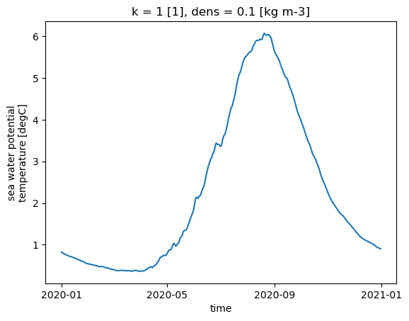
Finally, the full archive — every daily file from September 1992 to December 2024, covering over 30 years.
%%time
%%memit

ds_lazy = xhycom.open_mfdataset(DATA_PATH + "archm.*", grid=GRID_PATH, chunks={"time": 1})
peak memory: 36708.09 MiB, increment: 8188.00 MiB
CPU times: user 5min 4s, sys: 6.01 s, total: 5min 10s
Wall time: 5min 7s
ds_lazy
<xarray.Dataset> Size: 38TB
Dimensions:     (y: 380, x: 400, time: 11805, k: 50, ki: 51)
Coordinates:
    lon         (y, x) float64 1MB dask.array<chunksize=(380, 400), meta=np.ndarray>
    lat         (y, x) float64 1MB dask.array<chunksize=(380, 400), meta=np.ndarray>
    lon_u       (y, x) float64 1MB dask.array<chunksize=(380, 400), meta=np.ndarray>
    lat_u       (y, x) float64 1MB dask.array<chunksize=(380, 400), meta=np.ndarray>
    lon_v       (y, x) float64 1MB dask.array<chunksize=(380, 400), meta=np.ndarray>
    lat_v       (y, x) float64 1MB dask.array<chunksize=(380, 400), meta=np.ndarray>
  * time        (time) object 94kB 1992-09-06 00:00:00 ... 2024-12-31 00:00:00
  * k           (k) int64 400B 1 2 3 4 5 6 7 8 9 ... 42 43 44 45 46 47 48 49 50
    dens        (k) float64 400B dask.array<chunksize=(50,), meta=np.ndarray>
  * ki          (ki) int64 408B 0 1 2 3 4 5 6 7 8 ... 42 43 44 45 46 47 48 49 50
Dimensions without coordinates: y, x
Data variables: (12/83)
    montg1      (time, y, x) float64 14GB dask.array<chunksize=(1, 380, 400), meta=np.ndarray>
    srfhgt      (time, y, x) float64 14GB dask.array<chunksize=(1, 380, 400), meta=np.ndarray>
    oneta       (time, y, x) float64 14GB dask.array<chunksize=(1, 380, 400), meta=np.ndarray>
    surflx      (time, y, x) float64 14GB dask.array<chunksize=(1, 380, 400), meta=np.ndarray>
    wtrflx      (time, y, x) float64 14GB dask.array<chunksize=(1, 380, 400), meta=np.ndarray>
    salflx      (time, y, x) float64 14GB dask.array<chunksize=(1, 380, 400), meta=np.ndarray>
    ...          ...
    CO2_wind    (time, y, x) float64 14GB dask.array<chunksize=(1, 380, 400), meta=np.ndarray>
    ECO_bots    (time, y, x) float64 14GB dask.array<chunksize=(1, 380, 400), meta=np.ndarray>
    surface__1  (time, y, x) float64 14GB dask.array<chunksize=(1, 380, 400), meta=np.ndarray>
    surface__2  (time, y, x) float64 14GB dask.array<chunksize=(1, 380, 400), meta=np.ndarray>
    si_u        (time, y, x) float64 14GB dask.array<chunksize=(1, 380, 400), meta=np.ndarray>
    si_v        (time, y, x) float64 14GB dask.array<chunksize=(1, 380, 400), meta=np.ndarray>
Attributes:
    iversn:   23
    iexpt:    28
yrflag: 3- y: 380
- x: 400
- time: 11805
- k: 50
- ki: 51
- lon(y, x)float64dask.array<chunksize=(380, 400), meta=np.ndarray>
- long_name :
- longitude (T-point)
- units :
- degrees_east
- standard_name :
- longitude
Array Chunk Bytes 1.16 MiB 1.16 MiB Shape (380, 400) (380, 400) Dask graph 1 chunks in 1 graph layer Data type float64 numpy.ndarray - lat(y, x)float64dask.array<chunksize=(380, 400), meta=np.ndarray>
- long_name :
- latitude (T-point)
- units :
- degrees_north
- standard_name :
- latitude
Array Chunk Bytes 1.16 MiB 1.16 MiB Shape (380, 400) (380, 400) Dask graph 1 chunks in 1 graph layer Data type float64 numpy.ndarray - lon_u(y, x)float64dask.array<chunksize=(380, 400), meta=np.ndarray>
- long_name :
- longitude (U-point)
- units :
- degrees_east
Array Chunk Bytes 1.16 MiB 1.16 MiB Shape (380, 400) (380, 400) Dask graph 1 chunks in 1 graph layer Data type float64 numpy.ndarray - lat_u(y, x)float64dask.array<chunksize=(380, 400), meta=np.ndarray>
- long_name :
- latitude (U-point)
- units :
- degrees_north
Array Chunk Bytes 1.16 MiB 1.16 MiB Shape (380, 400) (380, 400) Dask graph 1 chunks in 1 graph layer Data type float64 numpy.ndarray - lon_v(y, x)float64dask.array<chunksize=(380, 400), meta=np.ndarray>
- long_name :
- longitude (V-point)
- units :
- degrees_east
Array Chunk Bytes 1.16 MiB 1.16 MiB Shape (380, 400) (380, 400) Dask graph 1 chunks in 1 graph layer Data type float64 numpy.ndarray - lat_v(y, x)float64dask.array<chunksize=(380, 400), meta=np.ndarray>
- long_name :
- latitude (V-point)
- units :
- degrees_north
Array Chunk Bytes 1.16 MiB 1.16 MiB Shape (380, 400) (380, 400) Dask graph 1 chunks in 1 graph layer Data type float64 numpy.ndarray - time(time)object1992-09-06 00:00:00 ... 2024-12-...
- long_name :
- time
- axis :
- T
array([cftime.DatetimeGregorian(1992, 9, 6, 0, 0, 0, 0, has_year_zero=False), cftime.DatetimeGregorian(1992, 9, 7, 0, 0, 0, 0, has_year_zero=False), cftime.DatetimeGregorian(1992, 9, 8, 0, 0, 0, 0, has_year_zero=False), ..., cftime.DatetimeGregorian(2024, 12, 29, 0, 0, 0, 0, has_year_zero=False), cftime.DatetimeGregorian(2024, 12, 30, 0, 0, 0, 0, has_year_zero=False), cftime.DatetimeGregorian(2024, 12, 31, 0, 0, 0, 0, has_year_zero=False)], shape=(11805,), dtype=object) - k(k)int641 2 3 4 5 6 7 ... 45 46 47 48 49 50
- long_name :
- layer index
- units :
- 1
- axis :
- Z
array([ 1, 2, 3, 4, 5, 6, 7, 8, 9, 10, 11, 12, 13, 14, 15, 16, 17, 18, 19, 20, 21, 22, 23, 24, 25, 26, 27, 28, 29, 30, 31, 32, 33, 34, 35, 36, 37, 38, 39, 40, 41, 42, 43, 44, 45, 46, 47, 48, 49, 50]) - dens(k)float64dask.array<chunksize=(50,), meta=np.ndarray>
- long_name :
- target sigma-2 layer density
- units :
- kg m-3
Array Chunk Bytes 400 B 400 B Shape (50,) (50,) Dask graph 1 chunks in 1 graph layer Data type float64 numpy.ndarray - ki(ki)int640 1 2 3 4 5 6 ... 45 46 47 48 49 50
- long_name :
- layer interface index
- units :
- 1
- axis :
- Z
array([ 0,  1,  2,  3,  4,  5,  6,  7,  8,  9, 10, 11, 12, 13, 14, 15, 16, 17,
       18, 19, 20, 21, 22, 23, 24, 25, 26, 27, 28, 29, 30, 31, 32, 33, 34, 35,
       36, 37, 38, 39, 40, 41, 42, 43, 44, 45, 46, 47, 48, 49, 50])
- montg1(time, y, x)float64dask.array<chunksize=(1, 380, 400), meta=np.ndarray>
- long_name :
- Montgomery potential
- units :
- m2 s-2
Array Chunk Bytes 13.37 GiB 1.16 MiB Shape (11805, 380, 400) (1, 380, 400) Dask graph 11805 chunks in 23611 graph layers Data type float64 numpy.ndarray - srfhgt(time, y, x)float64dask.array<chunksize=(1, 380, 400), meta=np.ndarray>
- long_name :
- sea surface height
- units :
- Pa
Array Chunk Bytes 13.37 GiB 1.16 MiB Shape (11805, 380, 400) (1, 380, 400) Dask graph 11805 chunks in 23611 graph layers Data type float64 numpy.ndarray - oneta(time, y, x)float64dask.array<chunksize=(1, 380, 400), meta=np.ndarray>
- long_name :
- free surface elevation
- units :
- m
Array Chunk Bytes 13.37 GiB 1.16 MiB Shape (11805, 380, 400) (1, 380, 400) Dask graph 11805 chunks in 23611 graph layers Data type float64 numpy.ndarray - surflx(time, y, x)float64dask.array<chunksize=(1, 380, 400), meta=np.ndarray>
- long_name :
- net surface heat flux
- units :
- W m-2
Array Chunk Bytes 13.37 GiB 1.16 MiB Shape (11805, 380, 400) (1, 380, 400) Dask graph 11805 chunks in 23611 graph layers Data type float64 numpy.ndarray - wtrflx(time, y, x)float64dask.array<chunksize=(1, 380, 400), meta=np.ndarray>
- long_name :
- net surface freshwater flux
- units :
- m s-1
Array Chunk Bytes 13.37 GiB 1.16 MiB Shape (11805, 380, 400) (1, 380, 400) Dask graph 11805 chunks in 23611 graph layers Data type float64 numpy.ndarray - salflx(time, y, x)float64dask.array<chunksize=(1, 380, 400), meta=np.ndarray>
- long_name :
- surface salt flux
- units :
- PSU m s-1
Array Chunk Bytes 13.37 GiB 1.16 MiB Shape (11805, 380, 400) (1, 380, 400) Dask graph 11805 chunks in 23611 graph layers Data type float64 numpy.ndarray - bl_dpth(time, y, x)float64dask.array<chunksize=(1, 380, 400), meta=np.ndarray>
- long_name :
- boundary layer depth
- units :
- Pa
Array Chunk Bytes 13.37 GiB 1.16 MiB Shape (11805, 380, 400) (1, 380, 400) Dask graph 11805 chunks in 23611 graph layers Data type float64 numpy.ndarray - mix_dpth(time, y, x)float64dask.array<chunksize=(1, 380, 400), meta=np.ndarray>
- long_name :
- mixed layer depth
- units :
- Pa
Array Chunk Bytes 13.37 GiB 1.16 MiB Shape (11805, 380, 400) (1, 380, 400) Dask graph 11805 chunks in 23611 graph layers Data type float64 numpy.ndarray - tmix(time, y, x)float64dask.array<chunksize=(1, 380, 400), meta=np.ndarray>
- long_name :
- mixed layer temperature
- units :
- degC
Array Chunk Bytes 13.37 GiB 1.16 MiB Shape (11805, 380, 400) (1, 380, 400) Dask graph 11805 chunks in 23611 graph layers Data type float64 numpy.ndarray - smix(time, y, x)float64dask.array<chunksize=(1, 380, 400), meta=np.ndarray>
- long_name :
- mixed layer salinity
- units :
- PSU
Array Chunk Bytes 13.37 GiB 1.16 MiB Shape (11805, 380, 400) (1, 380, 400) Dask graph 11805 chunks in 23611 graph layers Data type float64 numpy.ndarray - thmix(time, y, x)float64dask.array<chunksize=(1, 380, 400), meta=np.ndarray>
- long_name :
- mixed layer thickness
- units :
- Pa
Array Chunk Bytes 13.37 GiB 1.16 MiB Shape (11805, 380, 400) (1, 380, 400) Dask graph 11805 chunks in 23611 graph layers Data type float64 numpy.ndarray - umix(time, y, x)float64dask.array<chunksize=(1, 380, 400), meta=np.ndarray>
- long_name :
- mixed layer x velocity
- units :
- m s-1
Array Chunk Bytes 13.37 GiB 1.16 MiB Shape (11805, 380, 400) (1, 380, 400) Dask graph 11805 chunks in 23611 graph layers Data type float64 numpy.ndarray - vmix(time, y, x)float64dask.array<chunksize=(1, 380, 400), meta=np.ndarray>
- long_name :
- mixed layer y velocity
- units :
- m s-1
Array Chunk Bytes 13.37 GiB 1.16 MiB Shape (11805, 380, 400) (1, 380, 400) Dask graph 11805 chunks in 23611 graph layers Data type float64 numpy.ndarray - kemix(time, y, x)float64dask.array<chunksize=(1, 380, 400), meta=np.ndarray>
- long_name :
- mixed layer kinetic energy
- units :
- m2 s-2
Array Chunk Bytes 13.37 GiB 1.16 MiB Shape (11805, 380, 400) (1, 380, 400) Dask graph 11805 chunks in 23611 graph layers Data type float64 numpy.ndarray - covice(time, y, x)float64dask.array<chunksize=(1, 380, 400), meta=np.ndarray>
- long_name :
- sea ice coverage fraction
- units :
- 1
Array Chunk Bytes 13.37 GiB 1.16 MiB Shape (11805, 380, 400) (1, 380, 400) Dask graph 11805 chunks in 23611 graph layers Data type float64 numpy.ndarray - thkice(time, y, x)float64dask.array<chunksize=(1, 380, 400), meta=np.ndarray>
- long_name :
- sea ice thickness
- units :
- m
Array Chunk Bytes 13.37 GiB 1.16 MiB Shape (11805, 380, 400) (1, 380, 400) Dask graph 11805 chunks in 23611 graph layers Data type float64 numpy.ndarray - temice(time, y, x)float64dask.array<chunksize=(1, 380, 400), meta=np.ndarray>
- long_name :
- sea ice surface temperature
- units :
- degC
Array Chunk Bytes 13.37 GiB 1.16 MiB Shape (11805, 380, 400) (1, 380, 400) Dask graph 11805 chunks in 23611 graph layers Data type float64 numpy.ndarray - u_btrop(time, y, x)float64dask.array<chunksize=(1, 380, 400), meta=np.ndarray>
- long_name :
- barotropic x velocity
- units :
- m s-1
Array Chunk Bytes 13.37 GiB 1.16 MiB Shape (11805, 380, 400) (1, 380, 400) Dask graph 11805 chunks in 23611 graph layers Data type float64 numpy.ndarray - v_btrop(time, y, x)float64dask.array<chunksize=(1, 380, 400), meta=np.ndarray>
- long_name :
- barotropic y velocity
- units :
- m s-1
Array Chunk Bytes 13.37 GiB 1.16 MiB Shape (11805, 380, 400) (1, 380, 400) Dask graph 11805 chunks in 23611 graph layers Data type float64 numpy.ndarray - kebtrop(time, y, x)float64dask.array<chunksize=(1, 380, 400), meta=np.ndarray>
- long_name :
- barotropic kinetic energy
- units :
- m2 s-2
Array Chunk Bytes 13.37 GiB 1.16 MiB Shape (11805, 380, 400) (1, 380, 400) Dask graph 11805 chunks in 23611 graph layers Data type float64 numpy.ndarray - u-vel.(time, k, y, x)float64dask.array<chunksize=(1, 50, 380, 400), meta=np.ndarray>
- long_name :
- sea water x velocity
- units :
- m s-1
Array Chunk Bytes 668.45 GiB 57.98 MiB Shape (11805, 50, 380, 400) (1, 50, 380, 400) Dask graph 11805 chunks in 23611 graph layers Data type float64 numpy.ndarray - v-vel.(time, k, y, x)float64dask.array<chunksize=(1, 50, 380, 400), meta=np.ndarray>
- long_name :
- sea water y velocity
- units :
- m s-1
Array Chunk Bytes 668.45 GiB 57.98 MiB Shape (11805, 50, 380, 400) (1, 50, 380, 400) Dask graph 11805 chunks in 23611 graph layers Data type float64 numpy.ndarray - k.e.(time, k, y, x)float64dask.array<chunksize=(1, 50, 380, 400), meta=np.ndarray>
- long_name :
- kinetic energy
- units :
- m2 s-2
Array Chunk Bytes 668.45 GiB 57.98 MiB Shape (11805, 50, 380, 400) (1, 50, 380, 400) Dask graph 11805 chunks in 23611 graph layers Data type float64 numpy.ndarray - thknss(time, k, y, x)float64dask.array<chunksize=(1, 50, 380, 400), meta=np.ndarray>
- long_name :
- layer pressure thickness
- units :
- Pa
Array Chunk Bytes 668.45 GiB 57.98 MiB Shape (11805, 50, 380, 400) (1, 50, 380, 400) Dask graph 11805 chunks in 23611 graph layers Data type float64 numpy.ndarray - temp(time, k, y, x)float64dask.array<chunksize=(1, 50, 380, 400), meta=np.ndarray>
- long_name :
- sea water potential temperature
- units :
- degC
Array Chunk Bytes 668.45 GiB 57.98 MiB Shape (11805, 50, 380, 400) (1, 50, 380, 400) Dask graph 11805 chunks in 23611 graph layers Data type float64 numpy.ndarray - salin(time, k, y, x)float64dask.array<chunksize=(1, 50, 380, 400), meta=np.ndarray>
- long_name :
- sea water salinity
- units :
- PSU
Array Chunk Bytes 668.45 GiB 57.98 MiB Shape (11805, 50, 380, 400) (1, 50, 380, 400) Dask graph 11805 chunks in 23611 graph layers Data type float64 numpy.ndarray - density(time, k, y, x)float64dask.array<chunksize=(1, 50, 380, 400), meta=np.ndarray>
- long_name :
- sea water potential density (sigma-2)
- units :
- kg m-3
Array Chunk Bytes 668.45 GiB 57.98 MiB Shape (11805, 50, 380, 400) (1, 50, 380, 400) Dask graph 11805 chunks in 23611 graph layers Data type float64 numpy.ndarray - CO2_c(time, k, y, x)float64dask.array<chunksize=(1, 50, 380, 400), meta=np.ndarray>
- long_name :
- dissolved inorganic carbon
- units :
- mmol C m-3
Array Chunk Bytes 668.45 GiB 57.98 MiB Shape (11805, 50, 380, 400) (1, 50, 380, 400) Dask graph 11805 chunks in 23611 graph layers Data type float64 numpy.ndarray - CO2_TA(time, k, y, x)float64dask.array<chunksize=(1, 50, 380, 400), meta=np.ndarray>
- long_name :
- total alkalinity
- units :
- mmol eq m-3
Array Chunk Bytes 668.45 GiB 57.98 MiB Shape (11805, 50, 380, 400) (1, 50, 380, 400) Dask graph 11805 chunks in 23611 graph layers Data type float64 numpy.ndarray - ECO_no3(time, k, y, x)float64dask.array<chunksize=(1, 50, 380, 400), meta=np.ndarray>
- long_name :
- nitrate
- units :
- mmol N m-3
Array Chunk Bytes 668.45 GiB 57.98 MiB Shape (11805, 50, 380, 400) (1, 50, 380, 400) Dask graph 11805 chunks in 23611 graph layers Data type float64 numpy.ndarray - ECO_nh4(time, k, y, x)float64dask.array<chunksize=(1, 50, 380, 400), meta=np.ndarray>
- long_name :
- ammonium
- units :
- mmol N m-3
Array Chunk Bytes 668.45 GiB 57.98 MiB Shape (11805, 50, 380, 400) (1, 50, 380, 400) Dask graph 11805 chunks in 23611 graph layers Data type float64 numpy.ndarray - ECO_pho(time, k, y, x)float64dask.array<chunksize=(1, 50, 380, 400), meta=np.ndarray>
- long_name :
- phosphate
- units :
- mmol P m-3
Array Chunk Bytes 668.45 GiB 57.98 MiB Shape (11805, 50, 380, 400) (1, 50, 380, 400) Dask graph 11805 chunks in 23611 graph layers Data type float64 numpy.ndarray - ECO_sil(time, k, y, x)float64dask.array<chunksize=(1, 50, 380, 400), meta=np.ndarray>
- long_name :
- silicate
- units :
- mmol Si m-3
Array Chunk Bytes 668.45 GiB 57.98 MiB Shape (11805, 50, 380, 400) (1, 50, 380, 400) Dask graph 11805 chunks in 23611 graph layers Data type float64 numpy.ndarray - ECO_oxy(time, k, y, x)float64dask.array<chunksize=(1, 50, 380, 400), meta=np.ndarray>
- long_name :
- dissolved oxygen
- units :
- mmol O m-3
Array Chunk Bytes 668.45 GiB 57.98 MiB Shape (11805, 50, 380, 400) (1, 50, 380, 400) Dask graph 11805 chunks in 23611 graph layers Data type float64 numpy.ndarray - ECO_fla(time, k, y, x)float64dask.array<chunksize=(1, 50, 380, 400), meta=np.ndarray>
- long_name :
- flagellate carbon
- units :
- mmol C m-3
Array Chunk Bytes 668.45 GiB 57.98 MiB Shape (11805, 50, 380, 400) (1, 50, 380, 400) Dask graph 11805 chunks in 23611 graph layers Data type float64 numpy.ndarray - ECO_dia(time, k, y, x)float64dask.array<chunksize=(1, 50, 380, 400), meta=np.ndarray>
- long_name :
- diatom carbon
- units :
- mmol C m-3
Array Chunk Bytes 668.45 GiB 57.98 MiB Shape (11805, 50, 380, 400) (1, 50, 380, 400) Dask graph 11805 chunks in 23611 graph layers Data type float64 numpy.ndarray - ECO_ccl(time, k, y, x)float64dask.array<chunksize=(1, 50, 380, 400), meta=np.ndarray>
- long_name :
- coccolithophore carbon
- units :
- mmol C m-3
Array Chunk Bytes 668.45 GiB 57.98 MiB Shape (11805, 50, 380, 400) (1, 50, 380, 400) Dask graph 11805 chunks in 23611 graph layers Data type float64 numpy.ndarray - ECO_cclc(time, k, y, x)float64dask.array<chunksize=(1, 50, 380, 400), meta=np.ndarray>
- long_name :
- coccolithophore calcite carbon
- units :
- mmol C m-3
Array Chunk Bytes 668.45 GiB 57.98 MiB Shape (11805, 50, 380, 400) (1, 50, 380, 400) Dask graph 11805 chunks in 23611 graph layers Data type float64 numpy.ndarray - ECO_caco(time, k, y, x)float64dask.array<chunksize=(1, 50, 380, 400), meta=np.ndarray>
- long_name :
- particulate inorganic carbon (calcite)
- units :
- mmol C m-3
Array Chunk Bytes 668.45 GiB 57.98 MiB Shape (11805, 50, 380, 400) (1, 50, 380, 400) Dask graph 11805 chunks in 23611 graph layers Data type float64 numpy.ndarray - ECO_diac(time, k, y, x)float64dask.array<chunksize=(1, 50, 380, 400), meta=np.ndarray>
- long_name :
- diatom calcite carbon
- units :
- mmol C m-3
Array Chunk Bytes 668.45 GiB 57.98 MiB Shape (11805, 50, 380, 400) (1, 50, 380, 400) Dask graph 11805 chunks in 23611 graph layers Data type float64 numpy.ndarray - ECO_flac(time, k, y, x)float64dask.array<chunksize=(1, 50, 380, 400), meta=np.ndarray>
- long_name :
- flagellate calcite carbon
- units :
- mmol C m-3
Array Chunk Bytes 668.45 GiB 57.98 MiB Shape (11805, 50, 380, 400) (1, 50, 380, 400) Dask graph 11805 chunks in 23611 graph layers Data type float64 numpy.ndarray - ECO_micr(time, k, y, x)float64dask.array<chunksize=(1, 50, 380, 400), meta=np.ndarray>
- long_name :
- microzooplankton carbon
- units :
- mmol C m-3
Array Chunk Bytes 668.45 GiB 57.98 MiB Shape (11805, 50, 380, 400) (1, 50, 380, 400) Dask graph 11805 chunks in 23611 graph layers Data type float64 numpy.ndarray - ECO_meso(time, k, y, x)float64dask.array<chunksize=(1, 50, 380, 400), meta=np.ndarray>
- long_name :
- mesozooplankton carbon
- units :
- mmol C m-3
Array Chunk Bytes 668.45 GiB 57.98 MiB Shape (11805, 50, 380, 400) (1, 50, 380, 400) Dask graph 11805 chunks in 23611 graph layers Data type float64 numpy.ndarray - ECO_det(time, k, y, x)float64dask.array<chunksize=(1, 50, 380, 400), meta=np.ndarray>
- long_name :
- detritus carbon
- units :
- mmol C m-3
Array Chunk Bytes 668.45 GiB 57.98 MiB Shape (11805, 50, 380, 400) (1, 50, 380, 400) Dask graph 11805 chunks in 23611 graph layers Data type float64 numpy.ndarray - ECO_opa(time, k, y, x)float64dask.array<chunksize=(1, 50, 380, 400), meta=np.ndarray>
- long_name :
- opal (biogenic silica)
- units :
- mmol Si m-3
Array Chunk Bytes 668.45 GiB 57.98 MiB Shape (11805, 50, 380, 400) (1, 50, 380, 400) Dask graph 11805 chunks in 23611 graph layers Data type float64 numpy.ndarray - ECO_dom(time, k, y, x)float64dask.array<chunksize=(1, 50, 380, 400), meta=np.ndarray>
- long_name :
- dissolved organic matter carbon
- units :
- mmol C m-3
Array Chunk Bytes 668.45 GiB 57.98 MiB Shape (11805, 50, 380, 400) (1, 50, 380, 400) Dask graph 11805 chunks in 23611 graph layers Data type float64 numpy.ndarray - ECO_dsnk(time, k, y, x)float64dask.array<chunksize=(1, 50, 380, 400), meta=np.ndarray>
- long_name :
- detritus sinking flux
- units :
- mmol C m-2 s-1
Array Chunk Bytes 668.45 GiB 57.98 MiB Shape (11805, 50, 380, 400) (1, 50, 380, 400) Dask graph 11805 chunks in 23611 graph layers Data type float64 numpy.ndarray - CO2_pH(time, k, y, x)float64dask.array<chunksize=(1, 50, 380, 400), meta=np.ndarray>
- long_name :
- seawater pH
- units :
- 1
Array Chunk Bytes 668.45 GiB 57.98 MiB Shape (11805, 50, 380, 400) (1, 50, 380, 400) Dask graph 11805 chunks in 23611 graph layers Data type float64 numpy.ndarray - CO2_pCO2(time, k, y, x)float64dask.array<chunksize=(1, 50, 380, 400), meta=np.ndarray>
- long_name :
- partial pressure of CO2
- units :
- uatm
Array Chunk Bytes 668.45 GiB 57.98 MiB Shape (11805, 50, 380, 400) (1, 50, 380, 400) Dask graph 11805 chunks in 23611 graph layers Data type float64 numpy.ndarray - CO2_Carb_1(time, k, y, x)float64dask.array<chunksize=(1, 50, 380, 400), meta=np.ndarray>
- long_name :
- carbonate concentration
- units :
- mmol C m-3
Array Chunk Bytes 668.45 GiB 57.98 MiB Shape (11805, 50, 380, 400) (1, 50, 380, 400) Dask graph 11805 chunks in 23611 graph layers Data type float64 numpy.ndarray - CO2_BiCa(time, k, y, x)float64dask.array<chunksize=(1, 50, 380, 400), meta=np.ndarray>
- long_name :
- bicarbonate concentration
- units :
- mmol C m-3
Array Chunk Bytes 668.45 GiB 57.98 MiB Shape (11805, 50, 380, 400) (1, 50, 380, 400) Dask graph 11805 chunks in 23611 graph layers Data type float64 numpy.ndarray - CO2_Carb_2(time, k, y, x)float64dask.array<chunksize=(1, 50, 380, 400), meta=np.ndarray>
- long_name :
- carbonate concentration
- units :
- mmol C m-3
Array Chunk Bytes 668.45 GiB 57.98 MiB Shape (11805, 50, 380, 400) (1, 50, 380, 400) Dask graph 11805 chunks in 23611 graph layers Data type float64 numpy.ndarray - CO2_Om_c(time, k, y, x)float64dask.array<chunksize=(1, 50, 380, 400), meta=np.ndarray>
- long_name :
- calcite saturation state (Omega)
- units :
- 1
Array Chunk Bytes 668.45 GiB 57.98 MiB Shape (11805, 50, 380, 400) (1, 50, 380, 400) Dask graph 11805 chunks in 23611 graph layers Data type float64 numpy.ndarray - CO2_Om_a(time, k, y, x)float64dask.array<chunksize=(1, 50, 380, 400), meta=np.ndarray>
- long_name :
- aragonite saturation state (Omega)
- units :
- 1
Array Chunk Bytes 668.45 GiB 57.98 MiB Shape (11805, 50, 380, 400) (1, 50, 380, 400) Dask graph 11805 chunks in 23611 graph layers Data type float64 numpy.ndarray - ECO_prim(time, k, y, x)float64dask.array<chunksize=(1, 50, 380, 400), meta=np.ndarray>
- long_name :
- primary production
- units :
- mmol C m-3 s-1
Array Chunk Bytes 668.45 GiB 57.98 MiB Shape (11805, 50, 380, 400) (1, 50, 380, 400) Dask graph 11805 chunks in 23611 graph layers Data type float64 numpy.ndarray - ECO_secp(time, k, y, x)float64dask.array<chunksize=(1, 50, 380, 400), meta=np.ndarray>
- long_name :
- secondary production
- units :
- mmol C m-3 s-1
Array Chunk Bytes 668.45 GiB 57.98 MiB Shape (11805, 50, 380, 400) (1, 50, 380, 400) Dask graph 11805 chunks in 23611 graph layers Data type float64 numpy.ndarray - ECO_netp(time, k, y, x)float64dask.array<chunksize=(1, 50, 380, 400), meta=np.ndarray>
- long_name :
- net primary production
- units :
- mmol C m-3 s-1
Array Chunk Bytes 668.45 GiB 57.98 MiB Shape (11805, 50, 380, 400) (1, 50, 380, 400) Dask graph 11805 chunks in 23611 graph layers Data type float64 numpy.ndarray - ECO_parm(time, k, y, x)float64dask.array<chunksize=(1, 50, 380, 400), meta=np.ndarray>
- long_name :
- BGC parameter field
- units :
- 1
Array Chunk Bytes 668.45 GiB 57.98 MiB Shape (11805, 50, 380, 400) (1, 50, 380, 400) Dask graph 11805 chunks in 23611 graph layers Data type float64 numpy.ndarray - ECO_Nlim(time, k, y, x)float64dask.array<chunksize=(1, 50, 380, 400), meta=np.ndarray>
- long_name :
- nitrogen limitation factor
- units :
- 1
Array Chunk Bytes 668.45 GiB 57.98 MiB Shape (11805, 50, 380, 400) (1, 50, 380, 400) Dask graph 11805 chunks in 23611 graph layers Data type float64 numpy.ndarray - ECO_Plim(time, k, y, x)float64dask.array<chunksize=(1, 50, 380, 400), meta=np.ndarray>
- long_name :
- phosphorus limitation factor
- units :
- 1
Array Chunk Bytes 668.45 GiB 57.98 MiB Shape (11805, 50, 380, 400) (1, 50, 380, 400) Dask graph 11805 chunks in 23611 graph layers Data type float64 numpy.ndarray - ECO_Slim(time, k, y, x)float64dask.array<chunksize=(1, 50, 380, 400), meta=np.ndarray>
- long_name :
- silicate limitation factor
- units :
- 1
Array Chunk Bytes 668.45 GiB 57.98 MiB Shape (11805, 50, 380, 400) (1, 50, 380, 400) Dask graph 11805 chunks in 23611 graph layers Data type float64 numpy.ndarray - ECO_Llim(time, k, y, x)float64dask.array<chunksize=(1, 50, 380, 400), meta=np.ndarray>
- long_name :
- light limitation factor
- units :
- 1
Array Chunk Bytes 668.45 GiB 57.98 MiB Shape (11805, 50, 380, 400) (1, 50, 380, 400) Dask graph 11805 chunks in 23611 graph layers Data type float64 numpy.ndarray - ECO_deni(time, k, y, x)float64dask.array<chunksize=(1, 50, 380, 400), meta=np.ndarray>
- long_name :
- denitrification
- units :
- mmol N m-3 s-1
Array Chunk Bytes 668.45 GiB 57.98 MiB Shape (11805, 50, 380, 400) (1, 50, 380, 400) Dask graph 11805 chunks in 23611 graph layers Data type float64 numpy.ndarray - ECO_snks(time, k, y, x)float64dask.array<chunksize=(1, 50, 380, 400), meta=np.ndarray>
- long_name :
- sinking rate
- units :
- m d-1
Array Chunk Bytes 668.45 GiB 57.98 MiB Shape (11805, 50, 380, 400) (1, 50, 380, 400) Dask graph 11805 chunks in 23611 graph layers Data type float64 numpy.ndarray - ECO_c2ch_1(time, k, y, x)float64dask.array<chunksize=(1, 50, 380, 400), meta=np.ndarray>
- long_name :
- carbon to chlorophyll ratio
- units :
- g C g-1 Chl
Array Chunk Bytes 668.45 GiB 57.98 MiB Shape (11805, 50, 380, 400) (1, 50, 380, 400) Dask graph 11805 chunks in 23611 graph layers Data type float64 numpy.ndarray - ECO_c2ch_2(time, k, y, x)float64dask.array<chunksize=(1, 50, 380, 400), meta=np.ndarray>
- long_name :
- carbon to chlorophyll ratio
- units :
- g C g-1 Chl
Array Chunk Bytes 668.45 GiB 57.98 MiB Shape (11805, 50, 380, 400) (1, 50, 380, 400) Dask graph 11805 chunks in 23611 graph layers Data type float64 numpy.ndarray - ECO_c2ch_3(time, k, y, x)float64dask.array<chunksize=(1, 50, 380, 400), meta=np.ndarray>
- long_name :
- carbon to chlorophyll ratio
- units :
- g C g-1 Chl
Array Chunk Bytes 668.45 GiB 57.98 MiB Shape (11805, 50, 380, 400) (1, 50, 380, 400) Dask graph 11805 chunks in 23611 graph layers Data type float64 numpy.ndarray - light_sw(time, k, y, x)float64dask.array<chunksize=(1, 50, 380, 400), meta=np.ndarray>
- long_name :
- shortwave irradiance in water
- units :
- W m-2
Array Chunk Bytes 668.45 GiB 57.98 MiB Shape (11805, 50, 380, 400) (1, 50, 380, 400) Dask graph 11805 chunks in 23611 graph layers Data type float64 numpy.ndarray - light_pa(time, ki, y, x)float64dask.array<chunksize=(1, 51, 380, 400), meta=np.ndarray>
- long_name :
- PAR irradiance
- units :
- W m-2
Array Chunk Bytes 681.82 GiB 59.14 MiB Shape (11805, 51, 380, 400) (1, 51, 380, 400) Dask graph 11805 chunks in 23611 graph layers Data type float64 numpy.ndarray - attenuat(time, k, y, x)float64dask.array<chunksize=(1, 50, 380, 400), meta=np.ndarray>
- long_name :
- light attenuation coefficient
- units :
- m-1
Array Chunk Bytes 668.45 GiB 57.98 MiB Shape (11805, 50, 380, 400) (1, 50, 380, 400) Dask graph 11805 chunks in 23611 graph layers Data type float64 numpy.ndarray - total_ch(time, k, y, x)float64dask.array<chunksize=(1, 50, 380, 400), meta=np.ndarray>
- long_name :
- total chlorophyll
- units :
- mg Chl m-3
Array Chunk Bytes 668.45 GiB 57.98 MiB Shape (11805, 50, 380, 400) (1, 50, 380, 400) Dask graph 11805 chunks in 23611 graph layers Data type float64 numpy.ndarray - total_ca(time, k, y, x)float64dask.array<chunksize=(1, 50, 380, 400), meta=np.ndarray>
- long_name :
- total carbon
- units :
- mmol C m-3
Array Chunk Bytes 668.45 GiB 57.98 MiB Shape (11805, 50, 380, 400) (1, 50, 380, 400) Dask graph 11805 chunks in 23611 graph layers Data type float64 numpy.ndarray - ECO_sed4(time, y, x)float64dask.array<chunksize=(1, 380, 400), meta=np.ndarray>
- long_name :
- sediment pool 4
- units :
- mmol m-2
Array Chunk Bytes 13.37 GiB 1.16 MiB Shape (11805, 380, 400) (1, 380, 400) Dask graph 11805 chunks in 23611 graph layers Data type float64 numpy.ndarray - ECO_sed1(time, y, x)float64dask.array<chunksize=(1, 380, 400), meta=np.ndarray>
- long_name :
- sediment pool 1
- units :
- mmol m-2
Array Chunk Bytes 13.37 GiB 1.16 MiB Shape (11805, 380, 400) (1, 380, 400) Dask graph 11805 chunks in 23611 graph layers Data type float64 numpy.ndarray - ECO_sed2(time, y, x)float64dask.array<chunksize=(1, 380, 400), meta=np.ndarray>
- long_name :
- sediment pool 2
- units :
- mmol m-2
Array Chunk Bytes 13.37 GiB 1.16 MiB Shape (11805, 380, 400) (1, 380, 400) Dask graph 11805 chunks in 23611 graph layers Data type float64 numpy.ndarray - ECO_sed3(time, y, x)float64dask.array<chunksize=(1, 380, 400), meta=np.ndarray>
- long_name :
- sediment pool 3
- units :
- mmol m-2
Array Chunk Bytes 13.37 GiB 1.16 MiB Shape (11805, 380, 400) (1, 380, 400) Dask graph 11805 chunks in 23611 graph layers Data type float64 numpy.ndarray - CO2_fair(time, y, x)float64dask.array<chunksize=(1, 380, 400), meta=np.ndarray>
- long_name :
- air-sea CO2 flux
- units :
- mmol C m-2 d-1
Array Chunk Bytes 13.37 GiB 1.16 MiB Shape (11805, 380, 400) (1, 380, 400) Dask graph 11805 chunks in 23611 graph layers Data type float64 numpy.ndarray - CO2_wind(time, y, x)float64dask.array<chunksize=(1, 380, 400), meta=np.ndarray>
- long_name :
- wind speed for gas exchange
- units :
- m s-1
Array Chunk Bytes 13.37 GiB 1.16 MiB Shape (11805, 380, 400) (1, 380, 400) Dask graph 11805 chunks in 23611 graph layers Data type float64 numpy.ndarray - ECO_bots(time, y, x)float64dask.array<chunksize=(1, 380, 400), meta=np.ndarray>
- long_name :
- bottom sediment flux
- units :
- 1
Array Chunk Bytes 13.37 GiB 1.16 MiB Shape (11805, 380, 400) (1, 380, 400) Dask graph 11805 chunks in 23611 graph layers Data type float64 numpy.ndarray - surface__1(time, y, x)float64dask.array<chunksize=(1, 380, 400), meta=np.ndarray>
Array Chunk Bytes 13.37 GiB 1.16 MiB Shape (11805, 380, 400) (1, 380, 400) Dask graph 11805 chunks in 23611 graph layers Data type float64 numpy.ndarray - surface__2(time, y, x)float64dask.array<chunksize=(1, 380, 400), meta=np.ndarray>
Array Chunk Bytes 13.37 GiB 1.16 MiB Shape (11805, 380, 400) (1, 380, 400) Dask graph 11805 chunks in 23611 graph layers Data type float64 numpy.ndarray - si_u(time, y, x)float64dask.array<chunksize=(1, 380, 400), meta=np.ndarray>
- long_name :
- sea ice x velocity
- units :
- m s-1
Array Chunk Bytes 13.37 GiB 1.16 MiB Shape (11805, 380, 400) (1, 380, 400) Dask graph 11805 chunks in 23611 graph layers Data type float64 numpy.ndarray - si_v(time, y, x)float64dask.array<chunksize=(1, 380, 400), meta=np.ndarray>
- long_name :
- sea ice y velocity
- units :
- m s-1
Array Chunk Bytes 13.37 GiB 1.16 MiB Shape (11805, 380, 400) (1, 380, 400) Dask graph 11805 chunks in 23611 graph layers Data type float64 numpy.ndarray
- iversn :
- 23
- iexpt :
- 28
- yrflag :
- 3
The Dataset spans 11,805 snapshots (1992–2024) and represents 38 TB of data on disk — none of which is in RAM yet.
The 8 GB memory increment is not field data: it is the Dask task graph — one deferred read task per variable per file. With 83 variables and 11,805 files that is roughly one million graph entries, each carrying the file path, record index, and function reference needed to read one array on demand. At ~8 KB of Python-object overhead per task, the graph itself costs gigabytes.
Tip
You can shrink the graph by passing variables=["temp", "salin", "srfhgt"] (only
those fields are added to the graph) or by using larger time chunks
(chunks={"time": 30}, 30× fewer tasks). Both cut the task count substantially —
but, as the benchmark at the end of this notebook shows, the open time and memory
drop only ~2×, not in proportion to the task count: parsing the 11,805 .b
headers is a fixed cost neither option avoids.
Why the open call can be slow#
With chunks={"time": 1} and many files, xhycom builds one Dask task per variable per file. For a 30-year daily archive with 83 variables that is roughly one million graph entries — each a Python object carrying a file path, record index, and function reference. At ~8 KB of overhead per task the graph alone costs gigabytes of RAM and takes minutes to construct.
There are two ways to shrink the graph:
Option A — larger time chunks#
chunks={"time": 1} means one Dask task reads one file. A larger value groups
multiple files into a single task, so the task count shrinks by that factor —
though, as the benchmark shows, the open time and graph memory fall much more
slowly than the task count does.
Important: this only works efficiently because xhycom builds the graph at
the requested granularity — it is not equivalent to opening with
chunks={"time": 1} and then calling .rechunk(), which would add a
second layer of tasks and make things worse.
|
tasks (83 vars, 11 805 files) |
files read per task |
graph memory (measured) |
|---|---|---|---|
|
~980 k |
1 |
8.0 GiB |
|
~33 k |
30 |
3.9 GiB |
A 30× drop in tasks buys only a ~2× drop in memory (and in open time): the fixed
cost of parsing every .b header dominates. Choose a chunk size that fits your
typical access pattern. If you always process a full month of daily data at once,
{"time": 30} is a natural choice — but note that accessing any single time step
will then cause Dask to read the entire 30-file chunk.
%%time
%%memit

# 30-day chunks: 30× fewer tasks, 30× smaller graph
ds_chunked = xhycom.open_mfdataset(DATA_PATH + "archm.*", grid=GRID_PATH, chunks={"time": 30})
peak memory: 38000.27 MiB, increment: 3948.66 MiB
CPU times: user 3min 11s, sys: 4.31 s, total: 3min 16s
Wall time: 3min 14s
ds_chunked
<xarray.Dataset> Size: 38TB
Dimensions:     (y: 380, x: 400, time: 11805, k: 50, ki: 51)
Coordinates:
    lon         (y, x) float64 1MB dask.array<chunksize=(380, 400), meta=np.ndarray>
    lat         (y, x) float64 1MB dask.array<chunksize=(380, 400), meta=np.ndarray>
    lon_u       (y, x) float64 1MB dask.array<chunksize=(380, 400), meta=np.ndarray>
    lat_u       (y, x) float64 1MB dask.array<chunksize=(380, 400), meta=np.ndarray>
    lon_v       (y, x) float64 1MB dask.array<chunksize=(380, 400), meta=np.ndarray>
    lat_v       (y, x) float64 1MB dask.array<chunksize=(380, 400), meta=np.ndarray>
  * time        (time) object 94kB 1992-09-06 00:00:00 ... 2024-12-31 00:00:00
  * k           (k) int64 400B 1 2 3 4 5 6 7 8 9 ... 42 43 44 45 46 47 48 49 50
    dens        (k) float64 400B dask.array<chunksize=(50,), meta=np.ndarray>
  * ki          (ki) int64 408B 0 1 2 3 4 5 6 7 8 ... 42 43 44 45 46 47 48 49 50
Dimensions without coordinates: y, x
Data variables: (12/83)
    montg1      (time, y, x) float64 14GB dask.array<chunksize=(30, 380, 400), meta=np.ndarray>
    srfhgt      (time, y, x) float64 14GB dask.array<chunksize=(30, 380, 400), meta=np.ndarray>
    oneta       (time, y, x) float64 14GB dask.array<chunksize=(30, 380, 400), meta=np.ndarray>
    surflx      (time, y, x) float64 14GB dask.array<chunksize=(30, 380, 400), meta=np.ndarray>
    wtrflx      (time, y, x) float64 14GB dask.array<chunksize=(30, 380, 400), meta=np.ndarray>
    salflx      (time, y, x) float64 14GB dask.array<chunksize=(30, 380, 400), meta=np.ndarray>
    ...          ...
    CO2_wind    (time, y, x) float64 14GB dask.array<chunksize=(30, 380, 400), meta=np.ndarray>
    ECO_bots    (time, y, x) float64 14GB dask.array<chunksize=(30, 380, 400), meta=np.ndarray>
    surface__1  (time, y, x) float64 14GB dask.array<chunksize=(30, 380, 400), meta=np.ndarray>
    surface__2  (time, y, x) float64 14GB dask.array<chunksize=(30, 380, 400), meta=np.ndarray>
    si_u        (time, y, x) float64 14GB dask.array<chunksize=(30, 380, 400), meta=np.ndarray>
    si_v        (time, y, x) float64 14GB dask.array<chunksize=(30, 380, 400), meta=np.ndarray>
Attributes:
    iversn:   23
    iexpt:    28
yrflag: 3- y: 380
- x: 400
- time: 11805
- k: 50
- ki: 51
- lon(y, x)float64dask.array<chunksize=(380, 400), meta=np.ndarray>
- long_name :
- longitude (T-point)
- units :
- degrees_east
- standard_name :
- longitude
Array Chunk Bytes 1.16 MiB 1.16 MiB Shape (380, 400) (380, 400) Dask graph 1 chunks in 1 graph layer Data type float64 numpy.ndarray - lat(y, x)float64dask.array<chunksize=(380, 400), meta=np.ndarray>
- long_name :
- latitude (T-point)
- units :
- degrees_north
- standard_name :
- latitude
Array Chunk Bytes 1.16 MiB 1.16 MiB Shape (380, 400) (380, 400) Dask graph 1 chunks in 1 graph layer Data type float64 numpy.ndarray - lon_u(y, x)float64dask.array<chunksize=(380, 400), meta=np.ndarray>
- long_name :
- longitude (U-point)
- units :
- degrees_east
Array Chunk Bytes 1.16 MiB 1.16 MiB Shape (380, 400) (380, 400) Dask graph 1 chunks in 1 graph layer Data type float64 numpy.ndarray - lat_u(y, x)float64dask.array<chunksize=(380, 400), meta=np.ndarray>
- long_name :
- latitude (U-point)
- units :
- degrees_north
Array Chunk Bytes 1.16 MiB 1.16 MiB Shape (380, 400) (380, 400) Dask graph 1 chunks in 1 graph layer Data type float64 numpy.ndarray - lon_v(y, x)float64dask.array<chunksize=(380, 400), meta=np.ndarray>
- long_name :
- longitude (V-point)
- units :
- degrees_east
Array Chunk Bytes 1.16 MiB 1.16 MiB Shape (380, 400) (380, 400) Dask graph 1 chunks in 1 graph layer Data type float64 numpy.ndarray - lat_v(y, x)float64dask.array<chunksize=(380, 400), meta=np.ndarray>
- long_name :
- latitude (V-point)
- units :
- degrees_north
Array Chunk Bytes 1.16 MiB 1.16 MiB Shape (380, 400) (380, 400) Dask graph 1 chunks in 1 graph layer Data type float64 numpy.ndarray - time(time)object1992-09-06 00:00:00 ... 2024-12-...
- long_name :
- time
- axis :
- T
array([cftime.DatetimeGregorian(1992, 9, 6, 0, 0, 0, 0, has_year_zero=False), cftime.DatetimeGregorian(1992, 9, 7, 0, 0, 0, 0, has_year_zero=False), cftime.DatetimeGregorian(1992, 9, 8, 0, 0, 0, 0, has_year_zero=False), ..., cftime.DatetimeGregorian(2024, 12, 29, 0, 0, 0, 0, has_year_zero=False), cftime.DatetimeGregorian(2024, 12, 30, 0, 0, 0, 0, has_year_zero=False), cftime.DatetimeGregorian(2024, 12, 31, 0, 0, 0, 0, has_year_zero=False)], shape=(11805,), dtype=object) - k(k)int641 2 3 4 5 6 7 ... 45 46 47 48 49 50
- long_name :
- layer index
- units :
- 1
- axis :
- Z
array([ 1, 2, 3, 4, 5, 6, 7, 8, 9, 10, 11, 12, 13, 14, 15, 16, 17, 18, 19, 20, 21, 22, 23, 24, 25, 26, 27, 28, 29, 30, 31, 32, 33, 34, 35, 36, 37, 38, 39, 40, 41, 42, 43, 44, 45, 46, 47, 48, 49, 50]) - dens(k)float64dask.array<chunksize=(50,), meta=np.ndarray>
- long_name :
- target sigma-2 layer density
- units :
- kg m-3
Array Chunk Bytes 400 B 400 B Shape (50,) (50,) Dask graph 1 chunks in 1 graph layer Data type float64 numpy.ndarray - ki(ki)int640 1 2 3 4 5 6 ... 45 46 47 48 49 50
- long_name :
- layer interface index
- units :
- 1
- axis :
- Z
array([ 0,  1,  2,  3,  4,  5,  6,  7,  8,  9, 10, 11, 12, 13, 14, 15, 16, 17,
       18, 19, 20, 21, 22, 23, 24, 25, 26, 27, 28, 29, 30, 31, 32, 33, 34, 35,
       36, 37, 38, 39, 40, 41, 42, 43, 44, 45, 46, 47, 48, 49, 50])
- montg1(time, y, x)float64dask.array<chunksize=(30, 380, 400), meta=np.ndarray>
- long_name :
- Montgomery potential
- units :
- m2 s-2
Array Chunk Bytes 13.37 GiB 34.79 MiB Shape (11805, 380, 400) (30, 380, 400) Dask graph 394 chunks in 789 graph layers Data type float64 numpy.ndarray - srfhgt(time, y, x)float64dask.array<chunksize=(30, 380, 400), meta=np.ndarray>
- long_name :
- sea surface height
- units :
- Pa
Array Chunk Bytes 13.37 GiB 34.79 MiB Shape (11805, 380, 400) (30, 380, 400) Dask graph 394 chunks in 789 graph layers Data type float64 numpy.ndarray - oneta(time, y, x)float64dask.array<chunksize=(30, 380, 400), meta=np.ndarray>
- long_name :
- free surface elevation
- units :
- m
Array Chunk Bytes 13.37 GiB 34.79 MiB Shape (11805, 380, 400) (30, 380, 400) Dask graph 394 chunks in 789 graph layers Data type float64 numpy.ndarray - surflx(time, y, x)float64dask.array<chunksize=(30, 380, 400), meta=np.ndarray>
- long_name :
- net surface heat flux
- units :
- W m-2
Array Chunk Bytes 13.37 GiB 34.79 MiB Shape (11805, 380, 400) (30, 380, 400) Dask graph 394 chunks in 789 graph layers Data type float64 numpy.ndarray - wtrflx(time, y, x)float64dask.array<chunksize=(30, 380, 400), meta=np.ndarray>
- long_name :
- net surface freshwater flux
- units :
- m s-1
Array Chunk Bytes 13.37 GiB 34.79 MiB Shape (11805, 380, 400) (30, 380, 400) Dask graph 394 chunks in 789 graph layers Data type float64 numpy.ndarray - salflx(time, y, x)float64dask.array<chunksize=(30, 380, 400), meta=np.ndarray>
- long_name :
- surface salt flux
- units :
- PSU m s-1
Array Chunk Bytes 13.37 GiB 34.79 MiB Shape (11805, 380, 400) (30, 380, 400) Dask graph 394 chunks in 789 graph layers Data type float64 numpy.ndarray - bl_dpth(time, y, x)float64dask.array<chunksize=(30, 380, 400), meta=np.ndarray>
- long_name :
- boundary layer depth
- units :
- Pa
Array Chunk Bytes 13.37 GiB 34.79 MiB Shape (11805, 380, 400) (30, 380, 400) Dask graph 394 chunks in 789 graph layers Data type float64 numpy.ndarray - mix_dpth(time, y, x)float64dask.array<chunksize=(30, 380, 400), meta=np.ndarray>
- long_name :
- mixed layer depth
- units :
- Pa
Array Chunk Bytes 13.37 GiB 34.79 MiB Shape (11805, 380, 400) (30, 380, 400) Dask graph 394 chunks in 789 graph layers Data type float64 numpy.ndarray - tmix(time, y, x)float64dask.array<chunksize=(30, 380, 400), meta=np.ndarray>
- long_name :
- mixed layer temperature
- units :
- degC
Array Chunk Bytes 13.37 GiB 34.79 MiB Shape (11805, 380, 400) (30, 380, 400) Dask graph 394 chunks in 789 graph layers Data type float64 numpy.ndarray - smix(time, y, x)float64dask.array<chunksize=(30, 380, 400), meta=np.ndarray>
- long_name :
- mixed layer salinity
- units :
- PSU
Array Chunk Bytes 13.37 GiB 34.79 MiB Shape (11805, 380, 400) (30, 380, 400) Dask graph 394 chunks in 789 graph layers Data type float64 numpy.ndarray - thmix(time, y, x)float64dask.array<chunksize=(30, 380, 400), meta=np.ndarray>
- long_name :
- mixed layer thickness
- units :
- Pa
Array Chunk Bytes 13.37 GiB 34.79 MiB Shape (11805, 380, 400) (30, 380, 400) Dask graph 394 chunks in 789 graph layers Data type float64 numpy.ndarray - umix(time, y, x)float64dask.array<chunksize=(30, 380, 400), meta=np.ndarray>
- long_name :
- mixed layer x velocity
- units :
- m s-1
Array Chunk Bytes 13.37 GiB 34.79 MiB Shape (11805, 380, 400) (30, 380, 400) Dask graph 394 chunks in 789 graph layers Data type float64 numpy.ndarray - vmix(time, y, x)float64dask.array<chunksize=(30, 380, 400), meta=np.ndarray>
- long_name :
- mixed layer y velocity
- units :
- m s-1
Array Chunk Bytes 13.37 GiB 34.79 MiB Shape (11805, 380, 400) (30, 380, 400) Dask graph 394 chunks in 789 graph layers Data type float64 numpy.ndarray - kemix(time, y, x)float64dask.array<chunksize=(30, 380, 400), meta=np.ndarray>
- long_name :
- mixed layer kinetic energy
- units :
- m2 s-2
Array Chunk Bytes 13.37 GiB 34.79 MiB Shape (11805, 380, 400) (30, 380, 400) Dask graph 394 chunks in 789 graph layers Data type float64 numpy.ndarray - covice(time, y, x)float64dask.array<chunksize=(30, 380, 400), meta=np.ndarray>
- long_name :
- sea ice coverage fraction
- units :
- 1
Array Chunk Bytes 13.37 GiB 34.79 MiB Shape (11805, 380, 400) (30, 380, 400) Dask graph 394 chunks in 789 graph layers Data type float64 numpy.ndarray - thkice(time, y, x)float64dask.array<chunksize=(30, 380, 400), meta=np.ndarray>
- long_name :
- sea ice thickness
- units :
- m
Array Chunk Bytes 13.37 GiB 34.79 MiB Shape (11805, 380, 400) (30, 380, 400) Dask graph 394 chunks in 789 graph layers Data type float64 numpy.ndarray - temice(time, y, x)float64dask.array<chunksize=(30, 380, 400), meta=np.ndarray>
- long_name :
- sea ice surface temperature
- units :
- degC
Array Chunk Bytes 13.37 GiB 34.79 MiB Shape (11805, 380, 400) (30, 380, 400) Dask graph 394 chunks in 789 graph layers Data type float64 numpy.ndarray - u_btrop(time, y, x)float64dask.array<chunksize=(30, 380, 400), meta=np.ndarray>
- long_name :
- barotropic x velocity
- units :
- m s-1
Array Chunk Bytes 13.37 GiB 34.79 MiB Shape (11805, 380, 400) (30, 380, 400) Dask graph 394 chunks in 789 graph layers Data type float64 numpy.ndarray - v_btrop(time, y, x)float64dask.array<chunksize=(30, 380, 400), meta=np.ndarray>
- long_name :
- barotropic y velocity
- units :
- m s-1
Array Chunk Bytes 13.37 GiB 34.79 MiB Shape (11805, 380, 400) (30, 380, 400) Dask graph 394 chunks in 789 graph layers Data type float64 numpy.ndarray - kebtrop(time, y, x)float64dask.array<chunksize=(30, 380, 400), meta=np.ndarray>
- long_name :
- barotropic kinetic energy
- units :
- m2 s-2
Array Chunk Bytes 13.37 GiB 34.79 MiB Shape (11805, 380, 400) (30, 380, 400) Dask graph 394 chunks in 789 graph layers Data type float64 numpy.ndarray - u-vel.(time, k, y, x)float64dask.array<chunksize=(30, 50, 380, 400), meta=np.ndarray>
- long_name :
- sea water x velocity
- units :
- m s-1
Array Chunk Bytes 668.45 GiB 1.70 GiB Shape (11805, 50, 380, 400) (30, 50, 380, 400) Dask graph 394 chunks in 789 graph layers Data type float64 numpy.ndarray - v-vel.(time, k, y, x)float64dask.array<chunksize=(30, 50, 380, 400), meta=np.ndarray>
- long_name :
- sea water y velocity
- units :
- m s-1
Array Chunk Bytes 668.45 GiB 1.70 GiB Shape (11805, 50, 380, 400) (30, 50, 380, 400) Dask graph 394 chunks in 789 graph layers Data type float64 numpy.ndarray - k.e.(time, k, y, x)float64dask.array<chunksize=(30, 50, 380, 400), meta=np.ndarray>
- long_name :
- kinetic energy
- units :
- m2 s-2
Array Chunk Bytes 668.45 GiB 1.70 GiB Shape (11805, 50, 380, 400) (30, 50, 380, 400) Dask graph 394 chunks in 789 graph layers Data type float64 numpy.ndarray - thknss(time, k, y, x)float64dask.array<chunksize=(30, 50, 380, 400), meta=np.ndarray>
- long_name :
- layer pressure thickness
- units :
- Pa
Array Chunk Bytes 668.45 GiB 1.70 GiB Shape (11805, 50, 380, 400) (30, 50, 380, 400) Dask graph 394 chunks in 789 graph layers Data type float64 numpy.ndarray - temp(time, k, y, x)float64dask.array<chunksize=(30, 50, 380, 400), meta=np.ndarray>
- long_name :
- sea water potential temperature
- units :
- degC
Array Chunk Bytes 668.45 GiB 1.70 GiB Shape (11805, 50, 380, 400) (30, 50, 380, 400) Dask graph 394 chunks in 789 graph layers Data type float64 numpy.ndarray - salin(time, k, y, x)float64dask.array<chunksize=(30, 50, 380, 400), meta=np.ndarray>
- long_name :
- sea water salinity
- units :
- PSU
Array Chunk Bytes 668.45 GiB 1.70 GiB Shape (11805, 50, 380, 400) (30, 50, 380, 400) Dask graph 394 chunks in 789 graph layers Data type float64 numpy.ndarray - density(time, k, y, x)float64dask.array<chunksize=(30, 50, 380, 400), meta=np.ndarray>
- long_name :
- sea water potential density (sigma-2)
- units :
- kg m-3
Array Chunk Bytes 668.45 GiB 1.70 GiB Shape (11805, 50, 380, 400) (30, 50, 380, 400) Dask graph 394 chunks in 789 graph layers Data type float64 numpy.ndarray - CO2_c(time, k, y, x)float64dask.array<chunksize=(30, 50, 380, 400), meta=np.ndarray>
- long_name :
- dissolved inorganic carbon
- units :
- mmol C m-3
Array Chunk Bytes 668.45 GiB 1.70 GiB Shape (11805, 50, 380, 400) (30, 50, 380, 400) Dask graph 394 chunks in 789 graph layers Data type float64 numpy.ndarray - CO2_TA(time, k, y, x)float64dask.array<chunksize=(30, 50, 380, 400), meta=np.ndarray>
- long_name :
- total alkalinity
- units :
- mmol eq m-3
Array Chunk Bytes 668.45 GiB 1.70 GiB Shape (11805, 50, 380, 400) (30, 50, 380, 400) Dask graph 394 chunks in 789 graph layers Data type float64 numpy.ndarray - ECO_no3(time, k, y, x)float64dask.array<chunksize=(30, 50, 380, 400), meta=np.ndarray>
- long_name :
- nitrate
- units :
- mmol N m-3
Array Chunk Bytes 668.45 GiB 1.70 GiB Shape (11805, 50, 380, 400) (30, 50, 380, 400) Dask graph 394 chunks in 789 graph layers Data type float64 numpy.ndarray - ECO_nh4(time, k, y, x)float64dask.array<chunksize=(30, 50, 380, 400), meta=np.ndarray>
- long_name :
- ammonium
- units :
- mmol N m-3
Array Chunk Bytes 668.45 GiB 1.70 GiB Shape (11805, 50, 380, 400) (30, 50, 380, 400) Dask graph 394 chunks in 789 graph layers Data type float64 numpy.ndarray - ECO_pho(time, k, y, x)float64dask.array<chunksize=(30, 50, 380, 400), meta=np.ndarray>
- long_name :
- phosphate
- units :
- mmol P m-3
Array Chunk Bytes 668.45 GiB 1.70 GiB Shape (11805, 50, 380, 400) (30, 50, 380, 400) Dask graph 394 chunks in 789 graph layers Data type float64 numpy.ndarray - ECO_sil(time, k, y, x)float64dask.array<chunksize=(30, 50, 380, 400), meta=np.ndarray>
- long_name :
- silicate
- units :
- mmol Si m-3
Array Chunk Bytes 668.45 GiB 1.70 GiB Shape (11805, 50, 380, 400) (30, 50, 380, 400) Dask graph 394 chunks in 789 graph layers Data type float64 numpy.ndarray - ECO_oxy(time, k, y, x)float64dask.array<chunksize=(30, 50, 380, 400), meta=np.ndarray>
- long_name :
- dissolved oxygen
- units :
- mmol O m-3
Array Chunk Bytes 668.45 GiB 1.70 GiB Shape (11805, 50, 380, 400) (30, 50, 380, 400) Dask graph 394 chunks in 789 graph layers Data type float64 numpy.ndarray - ECO_fla(time, k, y, x)float64dask.array<chunksize=(30, 50, 380, 400), meta=np.ndarray>
- long_name :
- flagellate carbon
- units :
- mmol C m-3
Array Chunk Bytes 668.45 GiB 1.70 GiB Shape (11805, 50, 380, 400) (30, 50, 380, 400) Dask graph 394 chunks in 789 graph layers Data type float64 numpy.ndarray - ECO_dia(time, k, y, x)float64dask.array<chunksize=(30, 50, 380, 400), meta=np.ndarray>
- long_name :
- diatom carbon
- units :
- mmol C m-3
Array Chunk Bytes 668.45 GiB 1.70 GiB Shape (11805, 50, 380, 400) (30, 50, 380, 400) Dask graph 394 chunks in 789 graph layers Data type float64 numpy.ndarray - ECO_ccl(time, k, y, x)float64dask.array<chunksize=(30, 50, 380, 400), meta=np.ndarray>
- long_name :
- coccolithophore carbon
- units :
- mmol C m-3
Array Chunk Bytes 668.45 GiB 1.70 GiB Shape (11805, 50, 380, 400) (30, 50, 380, 400) Dask graph 394 chunks in 789 graph layers Data type float64 numpy.ndarray - ECO_cclc(time, k, y, x)float64dask.array<chunksize=(30, 50, 380, 400), meta=np.ndarray>
- long_name :
- coccolithophore calcite carbon
- units :
- mmol C m-3
Array Chunk Bytes 668.45 GiB 1.70 GiB Shape (11805, 50, 380, 400) (30, 50, 380, 400) Dask graph 394 chunks in 789 graph layers Data type float64 numpy.ndarray - ECO_caco(time, k, y, x)float64dask.array<chunksize=(30, 50, 380, 400), meta=np.ndarray>
- long_name :
- particulate inorganic carbon (calcite)
- units :
- mmol C m-3
Array Chunk Bytes 668.45 GiB 1.70 GiB Shape (11805, 50, 380, 400) (30, 50, 380, 400) Dask graph 394 chunks in 789 graph layers Data type float64 numpy.ndarray - ECO_diac(time, k, y, x)float64dask.array<chunksize=(30, 50, 380, 400), meta=np.ndarray>
- long_name :
- diatom calcite carbon
- units :
- mmol C m-3
Array Chunk Bytes 668.45 GiB 1.70 GiB Shape (11805, 50, 380, 400) (30, 50, 380, 400) Dask graph 394 chunks in 789 graph layers Data type float64 numpy.ndarray - ECO_flac(time, k, y, x)float64dask.array<chunksize=(30, 50, 380, 400), meta=np.ndarray>
- long_name :
- flagellate calcite carbon
- units :
- mmol C m-3
Array Chunk Bytes 668.45 GiB 1.70 GiB Shape (11805, 50, 380, 400) (30, 50, 380, 400) Dask graph 394 chunks in 789 graph layers Data type float64 numpy.ndarray - ECO_micr(time, k, y, x)float64dask.array<chunksize=(30, 50, 380, 400), meta=np.ndarray>
- long_name :
- microzooplankton carbon
- units :
- mmol C m-3
Array Chunk Bytes 668.45 GiB 1.70 GiB Shape (11805, 50, 380, 400) (30, 50, 380, 400) Dask graph 394 chunks in 789 graph layers Data type float64 numpy.ndarray - ECO_meso(time, k, y, x)float64dask.array<chunksize=(30, 50, 380, 400), meta=np.ndarray>
- long_name :
- mesozooplankton carbon
- units :
- mmol C m-3
Array Chunk Bytes 668.45 GiB 1.70 GiB Shape (11805, 50, 380, 400) (30, 50, 380, 400) Dask graph 394 chunks in 789 graph layers Data type float64 numpy.ndarray - ECO_det(time, k, y, x)float64dask.array<chunksize=(30, 50, 380, 400), meta=np.ndarray>
- long_name :
- detritus carbon
- units :
- mmol C m-3
Array Chunk Bytes 668.45 GiB 1.70 GiB Shape (11805, 50, 380, 400) (30, 50, 380, 400) Dask graph 394 chunks in 789 graph layers Data type float64 numpy.ndarray - ECO_opa(time, k, y, x)float64dask.array<chunksize=(30, 50, 380, 400), meta=np.ndarray>
- long_name :
- opal (biogenic silica)
- units :
- mmol Si m-3
Array Chunk Bytes 668.45 GiB 1.70 GiB Shape (11805, 50, 380, 400) (30, 50, 380, 400) Dask graph 394 chunks in 789 graph layers Data type float64 numpy.ndarray - ECO_dom(time, k, y, x)float64dask.array<chunksize=(30, 50, 380, 400), meta=np.ndarray>
- long_name :
- dissolved organic matter carbon
- units :
- mmol C m-3
Array Chunk Bytes 668.45 GiB 1.70 GiB Shape (11805, 50, 380, 400) (30, 50, 380, 400) Dask graph 394 chunks in 789 graph layers Data type float64 numpy.ndarray - ECO_dsnk(time, k, y, x)float64dask.array<chunksize=(30, 50, 380, 400), meta=np.ndarray>
- long_name :
- detritus sinking flux
- units :
- mmol C m-2 s-1
Array Chunk Bytes 668.45 GiB 1.70 GiB Shape (11805, 50, 380, 400) (30, 50, 380, 400) Dask graph 394 chunks in 789 graph layers Data type float64 numpy.ndarray - CO2_pH(time, k, y, x)float64dask.array<chunksize=(30, 50, 380, 400), meta=np.ndarray>
- long_name :
- seawater pH
- units :
- 1
Array Chunk Bytes 668.45 GiB 1.70 GiB Shape (11805, 50, 380, 400) (30, 50, 380, 400) Dask graph 394 chunks in 789 graph layers Data type float64 numpy.ndarray - CO2_pCO2(time, k, y, x)float64dask.array<chunksize=(30, 50, 380, 400), meta=np.ndarray>
- long_name :
- partial pressure of CO2
- units :
- uatm
Array Chunk Bytes 668.45 GiB 1.70 GiB Shape (11805, 50, 380, 400) (30, 50, 380, 400) Dask graph 394 chunks in 789 graph layers Data type float64 numpy.ndarray - CO2_Carb_1(time, k, y, x)float64dask.array<chunksize=(30, 50, 380, 400), meta=np.ndarray>
- long_name :
- carbonate concentration
- units :
- mmol C m-3
Array Chunk Bytes 668.45 GiB 1.70 GiB Shape (11805, 50, 380, 400) (30, 50, 380, 400) Dask graph 394 chunks in 789 graph layers Data type float64 numpy.ndarray - CO2_BiCa(time, k, y, x)float64dask.array<chunksize=(30, 50, 380, 400), meta=np.ndarray>
- long_name :
- bicarbonate concentration
- units :
- mmol C m-3
Array Chunk Bytes 668.45 GiB 1.70 GiB Shape (11805, 50, 380, 400) (30, 50, 380, 400) Dask graph 394 chunks in 789 graph layers Data type float64 numpy.ndarray - CO2_Carb_2(time, k, y, x)float64dask.array<chunksize=(30, 50, 380, 400), meta=np.ndarray>
- long_name :
- carbonate concentration
- units :
- mmol C m-3
Array Chunk Bytes 668.45 GiB 1.70 GiB Shape (11805, 50, 380, 400) (30, 50, 380, 400) Dask graph 394 chunks in 789 graph layers Data type float64 numpy.ndarray - CO2_Om_c(time, k, y, x)float64dask.array<chunksize=(30, 50, 380, 400), meta=np.ndarray>
- long_name :
- calcite saturation state (Omega)
- units :
- 1
Array Chunk Bytes 668.45 GiB 1.70 GiB Shape (11805, 50, 380, 400) (30, 50, 380, 400) Dask graph 394 chunks in 789 graph layers Data type float64 numpy.ndarray - CO2_Om_a(time, k, y, x)float64dask.array<chunksize=(30, 50, 380, 400), meta=np.ndarray>
- long_name :
- aragonite saturation state (Omega)
- units :
- 1
Array Chunk Bytes 668.45 GiB 1.70 GiB Shape (11805, 50, 380, 400) (30, 50, 380, 400) Dask graph 394 chunks in 789 graph layers Data type float64 numpy.ndarray - ECO_prim(time, k, y, x)float64dask.array<chunksize=(30, 50, 380, 400), meta=np.ndarray>
- long_name :
- primary production
- units :
- mmol C m-3 s-1
Array Chunk Bytes 668.45 GiB 1.70 GiB Shape (11805, 50, 380, 400) (30, 50, 380, 400) Dask graph 394 chunks in 789 graph layers Data type float64 numpy.ndarray - ECO_secp(time, k, y, x)float64dask.array<chunksize=(30, 50, 380, 400), meta=np.ndarray>
- long_name :
- secondary production
- units :
- mmol C m-3 s-1
Array Chunk Bytes 668.45 GiB 1.70 GiB Shape (11805, 50, 380, 400) (30, 50, 380, 400) Dask graph 394 chunks in 789 graph layers Data type float64 numpy.ndarray - ECO_netp(time, k, y, x)float64dask.array<chunksize=(30, 50, 380, 400), meta=np.ndarray>
- long_name :
- net primary production
- units :
- mmol C m-3 s-1
Array Chunk Bytes 668.45 GiB 1.70 GiB Shape (11805, 50, 380, 400) (30, 50, 380, 400) Dask graph 394 chunks in 789 graph layers Data type float64 numpy.ndarray - ECO_parm(time, k, y, x)float64dask.array<chunksize=(30, 50, 380, 400), meta=np.ndarray>
- long_name :
- BGC parameter field
- units :
- 1
Array Chunk Bytes 668.45 GiB 1.70 GiB Shape (11805, 50, 380, 400) (30, 50, 380, 400) Dask graph 394 chunks in 789 graph layers Data type float64 numpy.ndarray - ECO_Nlim(time, k, y, x)float64dask.array<chunksize=(30, 50, 380, 400), meta=np.ndarray>
- long_name :
- nitrogen limitation factor
- units :
- 1
Array Chunk Bytes 668.45 GiB 1.70 GiB Shape (11805, 50, 380, 400) (30, 50, 380, 400) Dask graph 394 chunks in 789 graph layers Data type float64 numpy.ndarray - ECO_Plim(time, k, y, x)float64dask.array<chunksize=(30, 50, 380, 400), meta=np.ndarray>
- long_name :
- phosphorus limitation factor
- units :
- 1
Array Chunk Bytes 668.45 GiB 1.70 GiB Shape (11805, 50, 380, 400) (30, 50, 380, 400) Dask graph 394 chunks in 789 graph layers Data type float64 numpy.ndarray - ECO_Slim(time, k, y, x)float64dask.array<chunksize=(30, 50, 380, 400), meta=np.ndarray>
- long_name :
- silicate limitation factor
- units :
- 1
Array Chunk Bytes 668.45 GiB 1.70 GiB Shape (11805, 50, 380, 400) (30, 50, 380, 400) Dask graph 394 chunks in 789 graph layers Data type float64 numpy.ndarray - ECO_Llim(time, k, y, x)float64dask.array<chunksize=(30, 50, 380, 400), meta=np.ndarray>
- long_name :
- light limitation factor
- units :
- 1
Array Chunk Bytes 668.45 GiB 1.70 GiB Shape (11805, 50, 380, 400) (30, 50, 380, 400) Dask graph 394 chunks in 789 graph layers Data type float64 numpy.ndarray - ECO_deni(time, k, y, x)float64dask.array<chunksize=(30, 50, 380, 400), meta=np.ndarray>
- long_name :
- denitrification
- units :
- mmol N m-3 s-1
Array Chunk Bytes 668.45 GiB 1.70 GiB Shape (11805, 50, 380, 400) (30, 50, 380, 400) Dask graph 394 chunks in 789 graph layers Data type float64 numpy.ndarray - ECO_snks(time, k, y, x)float64dask.array<chunksize=(30, 50, 380, 400), meta=np.ndarray>
- long_name :
- sinking rate
- units :
- m d-1
Array Chunk Bytes 668.45 GiB 1.70 GiB Shape (11805, 50, 380, 400) (30, 50, 380, 400) Dask graph 394 chunks in 789 graph layers Data type float64 numpy.ndarray - ECO_c2ch_1(time, k, y, x)float64dask.array<chunksize=(30, 50, 380, 400), meta=np.ndarray>
- long_name :
- carbon to chlorophyll ratio
- units :
- g C g-1 Chl
Array Chunk Bytes 668.45 GiB 1.70 GiB Shape (11805, 50, 380, 400) (30, 50, 380, 400) Dask graph 394 chunks in 789 graph layers Data type float64 numpy.ndarray - ECO_c2ch_2(time, k, y, x)float64dask.array<chunksize=(30, 50, 380, 400), meta=np.ndarray>
- long_name :
- carbon to chlorophyll ratio
- units :
- g C g-1 Chl
Array Chunk Bytes 668.45 GiB 1.70 GiB Shape (11805, 50, 380, 400) (30, 50, 380, 400) Dask graph 394 chunks in 789 graph layers Data type float64 numpy.ndarray - ECO_c2ch_3(time, k, y, x)float64dask.array<chunksize=(30, 50, 380, 400), meta=np.ndarray>
- long_name :
- carbon to chlorophyll ratio
- units :
- g C g-1 Chl
Array Chunk Bytes 668.45 GiB 1.70 GiB Shape (11805, 50, 380, 400) (30, 50, 380, 400) Dask graph 394 chunks in 789 graph layers Data type float64 numpy.ndarray - light_sw(time, k, y, x)float64dask.array<chunksize=(30, 50, 380, 400), meta=np.ndarray>
- long_name :
- shortwave irradiance in water
- units :
- W m-2
Array Chunk Bytes 668.45 GiB 1.70 GiB Shape (11805, 50, 380, 400) (30, 50, 380, 400) Dask graph 394 chunks in 789 graph layers Data type float64 numpy.ndarray - light_pa(time, ki, y, x)float64dask.array<chunksize=(30, 51, 380, 400), meta=np.ndarray>
- long_name :
- PAR irradiance
- units :
- W m-2
Array Chunk Bytes 681.82 GiB 1.73 GiB Shape (11805, 51, 380, 400) (30, 51, 380, 400) Dask graph 394 chunks in 789 graph layers Data type float64 numpy.ndarray - attenuat(time, k, y, x)float64dask.array<chunksize=(30, 50, 380, 400), meta=np.ndarray>
- long_name :
- light attenuation coefficient
- units :
- m-1
Array Chunk Bytes 668.45 GiB 1.70 GiB Shape (11805, 50, 380, 400) (30, 50, 380, 400) Dask graph 394 chunks in 789 graph layers Data type float64 numpy.ndarray - total_ch(time, k, y, x)float64dask.array<chunksize=(30, 50, 380, 400), meta=np.ndarray>
- long_name :
- total chlorophyll
- units :
- mg Chl m-3
Array Chunk Bytes 668.45 GiB 1.70 GiB Shape (11805, 50, 380, 400) (30, 50, 380, 400) Dask graph 394 chunks in 789 graph layers Data type float64 numpy.ndarray - total_ca(time, k, y, x)float64dask.array<chunksize=(30, 50, 380, 400), meta=np.ndarray>
- long_name :
- total carbon
- units :
- mmol C m-3
Array Chunk Bytes 668.45 GiB 1.70 GiB Shape (11805, 50, 380, 400) (30, 50, 380, 400) Dask graph 394 chunks in 789 graph layers Data type float64 numpy.ndarray - ECO_sed4(time, y, x)float64dask.array<chunksize=(30, 380, 400), meta=np.ndarray>
- long_name :
- sediment pool 4
- units :
- mmol m-2
Array Chunk Bytes 13.37 GiB 34.79 MiB Shape (11805, 380, 400) (30, 380, 400) Dask graph 394 chunks in 789 graph layers Data type float64 numpy.ndarray - ECO_sed1(time, y, x)float64dask.array<chunksize=(30, 380, 400), meta=np.ndarray>
- long_name :
- sediment pool 1
- units :
- mmol m-2
Array Chunk Bytes 13.37 GiB 34.79 MiB Shape (11805, 380, 400) (30, 380, 400) Dask graph 394 chunks in 789 graph layers Data type float64 numpy.ndarray - ECO_sed2(time, y, x)float64dask.array<chunksize=(30, 380, 400), meta=np.ndarray>
- long_name :
- sediment pool 2
- units :
- mmol m-2
Array Chunk Bytes 13.37 GiB 34.79 MiB Shape (11805, 380, 400) (30, 380, 400) Dask graph 394 chunks in 789 graph layers Data type float64 numpy.ndarray - ECO_sed3(time, y, x)float64dask.array<chunksize=(30, 380, 400), meta=np.ndarray>
- long_name :
- sediment pool 3
- units :
- mmol m-2
Array Chunk Bytes 13.37 GiB 34.79 MiB Shape (11805, 380, 400) (30, 380, 400) Dask graph 394 chunks in 789 graph layers Data type float64 numpy.ndarray - CO2_fair(time, y, x)float64dask.array<chunksize=(30, 380, 400), meta=np.ndarray>
- long_name :
- air-sea CO2 flux
- units :
- mmol C m-2 d-1
Array Chunk Bytes 13.37 GiB 34.79 MiB Shape (11805, 380, 400) (30, 380, 400) Dask graph 394 chunks in 789 graph layers Data type float64 numpy.ndarray - CO2_wind(time, y, x)float64dask.array<chunksize=(30, 380, 400), meta=np.ndarray>
- long_name :
- wind speed for gas exchange
- units :
- m s-1
Array Chunk Bytes 13.37 GiB 34.79 MiB Shape (11805, 380, 400) (30, 380, 400) Dask graph 394 chunks in 789 graph layers Data type float64 numpy.ndarray - ECO_bots(time, y, x)float64dask.array<chunksize=(30, 380, 400), meta=np.ndarray>
- long_name :
- bottom sediment flux
- units :
- 1
Array Chunk Bytes 13.37 GiB 34.79 MiB Shape (11805, 380, 400) (30, 380, 400) Dask graph 394 chunks in 789 graph layers Data type float64 numpy.ndarray - surface__1(time, y, x)float64dask.array<chunksize=(30, 380, 400), meta=np.ndarray>
Array Chunk Bytes 13.37 GiB 34.79 MiB Shape (11805, 380, 400) (30, 380, 400) Dask graph 394 chunks in 789 graph layers Data type float64 numpy.ndarray - surface__2(time, y, x)float64dask.array<chunksize=(30, 380, 400), meta=np.ndarray>
Array Chunk Bytes 13.37 GiB 34.79 MiB Shape (11805, 380, 400) (30, 380, 400) Dask graph 394 chunks in 789 graph layers Data type float64 numpy.ndarray - si_u(time, y, x)float64dask.array<chunksize=(30, 380, 400), meta=np.ndarray>
- long_name :
- sea ice x velocity
- units :
- m s-1
Array Chunk Bytes 13.37 GiB 34.79 MiB Shape (11805, 380, 400) (30, 380, 400) Dask graph 394 chunks in 789 graph layers Data type float64 numpy.ndarray - si_v(time, y, x)float64dask.array<chunksize=(30, 380, 400), meta=np.ndarray>
- long_name :
- sea ice y velocity
- units :
- m s-1
Array Chunk Bytes 13.37 GiB 34.79 MiB Shape (11805, 380, 400) (30, 380, 400) Dask graph 394 chunks in 789 graph layers Data type float64 numpy.ndarray
- iversn :
- 23
- iexpt :
- 28
- yrflag :
- 3
Option B — load only the variables you need#
The variables= parameter limits which fields are included in the Dataset —
unneeded variables are never added to the Dask graph, which trims the task count
in proportion to the number of variables kept. In practice, though, the open time
and graph memory fall much less than that (see the benchmark): parsing every file’s
.b header is a fixed cost paid regardless of how many variables you request.
%%time
%%memit

# Only 3 variables → ~35 k tasks instead of ~980 k
ds_vars = xhycom.open_mfdataset(DATA_PATH + "archm.*", grid=GRID_PATH, chunks={"time": 1}, variables=["temp", "salin", "srfhgt"])
peak memory: 38988.80 MiB, increment: 3649.22 MiB
CPU times: user 2min 46s, sys: 4.25 s, total: 2min 50s
Wall time: 2min 49s
ds_vars
<xarray.Dataset> Size: 1TB
Dimensions: (y: 380, x: 400, time: 11805, k: 50)
Coordinates:
lon (y, x) float64 1MB dask.array<chunksize=(380, 400), meta=np.ndarray>
lat (y, x) float64 1MB dask.array<chunksize=(380, 400), meta=np.ndarray>
* time (time) object 94kB 1992-09-06 00:00:00 ... 2024-12-31 00:00:00
* k (k) int64 400B 1 2 3 4 5 6 7 8 9 10 ... 42 43 44 45 46 47 48 49 50
dens (k) float64 400B dask.array<chunksize=(50,), meta=np.ndarray>
Dimensions without coordinates: y, x
Data variables:
srfhgt (time, y, x) float64 14GB dask.array<chunksize=(1, 380, 400), meta=np.ndarray>
temp (time, k, y, x) float64 718GB dask.array<chunksize=(1, 50, 380, 400), meta=np.ndarray>
salin (time, k, y, x) float64 718GB dask.array<chunksize=(1, 50, 380, 400), meta=np.ndarray>
Attributes:
iversn: 23
iexpt: 28
yrflag: 3- y: 380
- x: 400
- time: 11805
- k: 50
- lon(y, x)float64dask.array<chunksize=(380, 400), meta=np.ndarray>
- long_name :
- longitude (T-point)
- units :
- degrees_east
- standard_name :
- longitude
Array Chunk Bytes 1.16 MiB 1.16 MiB Shape (380, 400) (380, 400) Dask graph 1 chunks in 1 graph layer Data type float64 numpy.ndarray - lat(y, x)float64dask.array<chunksize=(380, 400), meta=np.ndarray>
- long_name :
- latitude (T-point)
- units :
- degrees_north
- standard_name :
- latitude
Array Chunk Bytes 1.16 MiB 1.16 MiB Shape (380, 400) (380, 400) Dask graph 1 chunks in 1 graph layer Data type float64 numpy.ndarray - time(time)object1992-09-06 00:00:00 ... 2024-12-...
- long_name :
- time
- axis :
- T
array([cftime.DatetimeGregorian(1992, 9, 6, 0, 0, 0, 0, has_year_zero=False), cftime.DatetimeGregorian(1992, 9, 7, 0, 0, 0, 0, has_year_zero=False), cftime.DatetimeGregorian(1992, 9, 8, 0, 0, 0, 0, has_year_zero=False), ..., cftime.DatetimeGregorian(2024, 12, 29, 0, 0, 0, 0, has_year_zero=False), cftime.DatetimeGregorian(2024, 12, 30, 0, 0, 0, 0, has_year_zero=False), cftime.DatetimeGregorian(2024, 12, 31, 0, 0, 0, 0, has_year_zero=False)], shape=(11805,), dtype=object) - k(k)int641 2 3 4 5 6 7 ... 45 46 47 48 49 50
- long_name :
- layer index
- units :
- 1
- axis :
- Z
array([ 1, 2, 3, 4, 5, 6, 7, 8, 9, 10, 11, 12, 13, 14, 15, 16, 17, 18, 19, 20, 21, 22, 23, 24, 25, 26, 27, 28, 29, 30, 31, 32, 33, 34, 35, 36, 37, 38, 39, 40, 41, 42, 43, 44, 45, 46, 47, 48, 49, 50]) - dens(k)float64dask.array<chunksize=(50,), meta=np.ndarray>
- long_name :
- target sigma-2 layer density
- units :
- kg m-3
Array Chunk Bytes 400 B 400 B Shape (50,) (50,) Dask graph 1 chunks in 1 graph layer Data type float64 numpy.ndarray
- srfhgt(time, y, x)float64dask.array<chunksize=(1, 380, 400), meta=np.ndarray>
- long_name :
- sea surface height
- units :
- Pa
Array Chunk Bytes 13.37 GiB 1.16 MiB Shape (11805, 380, 400) (1, 380, 400) Dask graph 11805 chunks in 23611 graph layers Data type float64 numpy.ndarray - temp(time, k, y, x)float64dask.array<chunksize=(1, 50, 380, 400), meta=np.ndarray>
- long_name :
- sea water potential temperature
- units :
- degC
Array Chunk Bytes 668.45 GiB 57.98 MiB Shape (11805, 50, 380, 400) (1, 50, 380, 400) Dask graph 11805 chunks in 23611 graph layers Data type float64 numpy.ndarray - salin(time, k, y, x)float64dask.array<chunksize=(1, 50, 380, 400), meta=np.ndarray>
- long_name :
- sea water salinity
- units :
- PSU
Array Chunk Bytes 668.45 GiB 57.98 MiB Shape (11805, 50, 380, 400) (1, 50, 380, 400) Dask graph 11805 chunks in 23611 graph layers Data type float64 numpy.ndarray
- iversn :
- 23
- iexpt :
- 28
- yrflag :
- 3
You can also combine both options A and B — variables= with chunks={"time": 30} — to get the maximum reduction in graph size.
%%time
%%memit
ds_vars = xhycom.open_mfdataset(DATA_PATH + "archm.*", grid=GRID_PATH, chunks={"time": 30}, variables=["temp", "salin", "srfhgt"])
peak memory: 39026.82 MiB, increment: 2698.10 MiB
CPU times: user 2min 53s, sys: 4.45 s, total: 2min 58s
Wall time: 2min 56s
%%time
%%memit
sst_mean = ds_lazy.temp.isel(k=0).mean(dim=["y", "x"]).compute()
peak memory: 36676.98 MiB, increment: 309.92 MiB
CPU times: user 8min 46s, sys: 3min 38s, total: 12min 25s
Wall time: 10min 15s
Wall time: ~10 min — streaming all 11,805 daily
.afiles to reduce surface temperature to a scalar time series. This is the same ~10 min you would get on 8 CPUs: the reduction is disk-bound, so the 256 cores here do not help (see the benchmark at the end of this notebook).Increment: ~12 GiB — not a single time step’s worth. With 256 threads, Dask keeps hundreds of
tempchunks in flight at once, and eachchunks={"time": 1}block still holds all 50 layers (~60 MB). At a few cores the same reduction needs only a few hundred MiB — the streaming advantage is a low-core-count phenomenon.
sst_mean.plot()
[<matplotlib.lines.Line2D at 0x153b1fdec3d0>]
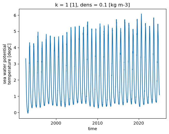
%%time
%%memit
ssh_mean = ds_lazy.srfhgt.mean(dim=["y", "x"]).compute()
peak memory: 36428.03 MiB, increment: 4.02 MiB
CPU times: user 2min 45s, sys: 6.81 s, total: 2min 52s
Wall time: 2min 41s
ssh_mean.plot()
[<matplotlib.lines.Line2D at 0x1539ebf35850>]
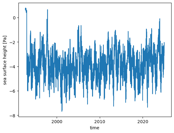
Regridding a time series#
Regridding HYCOM’s curvilinear, hybrid-coordinate output onto a regular lon/lat/depth grid is the other heavy operation you’ll run on these archives. See Regridding for what it does and the full set of options — here we only time it, to gauge how many CPUs the task is worth.
The remap has two costs that scale very differently:
Generating the weights — building the xESMF weight matrix. Serial work that depends only on the source and target grids, so it does not speed up with more cores;
weights=Truecaches it to disk so you pay it once.Applying the weights — the actual remap, deferred and streamed one time chunk at a time, exactly like the
.compute()reductions above, so it parallelises across cores the same way.
We regrid one year onto the GLORYS grid and reduce surface salinity to a time-mean — a reproducible workload that streams every time chunk through the cached weights. The benchmark section below adds a regridding row so you can track both costs across CPU counts.
# GLORYS target grid (regular lon/lat/depth + land mask); see the regridding notebook.
GLORYS_PATH = "/nird/datapeak/NS9481K/MERCATOR_DATA/REGULAR_GRID_COORD/GLO-MFC_001_030_mask_bathy.nc"
%%time
%%memit
# One year, lazy; postprocess=True puts thicknesses/SSH in metres for the vertical step.
ds_year = xhycom.open_mfdataset(DATA_PATH + "archm.2020*", grid=GRID_PATH,
chunks={"time": 1}, postprocess=True)
peak memory: 36532.11 MiB, increment: 112.77 MiB
CPU times: user 21.1 s, sys: 616 ms, total: 21.7 s
Wall time: 21.9 s
%%time
%%memit
# Build the regrid: generates (and caches) the xESMF weight matrix — the serial,
# CPU-independent cost. The remap itself stays lazy. See regridding.ipynb.
ds_g = xhycom.regrid(ds_year, target=GLORYS_PATH, grid=GRID_PATH, weights=True)
peak memory: 54365.43 MiB, increment: 17861.99 MiB
CPU times: user 44.4 s, sys: 10.7 s, total: 55.1 s
Wall time: 59.4 s
%%time
%%memit
# Apply the weights: streams every time chunk through the remap — the part that
# scales with CPU count, like the SST/SSH means above.
smean_g = ds_g["salin"].isel(depth=0).mean("time").compute()
peak memory: 93595.64 MiB, increment: 42279.75 MiB
CPU times: user 50min 20s, sys: 8min 37s, total: 58min 58s
Wall time: 7min 49s
smean_g.plot()
<matplotlib.collections.QuadMesh at 0x153c0e49a110>
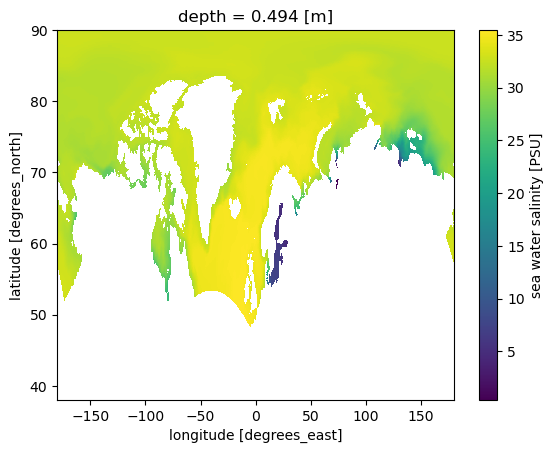
Benchmark: what scales with CPU count, and what doesn’t#
These cells were profiled on Olivia’s small partition (--partition=small —
the Open OnDemand default, a shared partial-node allocation) at four core counts:
1, 4, 8, and 256 CPUs. Unless a row says otherwise, the data are opened with
the notebook’s default lazy chunking — chunks={"time": 1} with the layer
dimension left whole (k: -1) — so each chunk is a single snapshot spanning all
50 layers. The headline result: most of the cost does not come down with more
cores. Only the read-bound .compute() reductions speed up, and only up to a
point — past which extra threads just consume more memory.
Independent of CPU count — opening data and building weights#
open_mfdataset(..., chunks=...) builds the Dask graph with serial Python work:
it parses one .b header per file and creates one task per variable per chunk.
Its wall time and its memory are set by the number of files and tasks, not by
the core count — across 1–256 CPUs both stayed within a few percent. Building the
regrid weight matrix is likewise serial and grid-dependent, so it doesn’t scale
with cores either (and weights=True caches it, so it’s a one-off).
Operation |
Wall time |
Memory increment |
|---|---|---|
Open 9 files, eager (no |
~1 min 15 s |
53 GiB |
Open 9 files, lazy ( |
~0.5 s |
~90 MiB |
Open 1 year, lazy (366 files) |
~9 s |
~400 MiB |
Open full archive (11 805 files), |
~5 min |
8.0 GiB |
Open full archive, |
~3 min |
3.9 GiB |
Open full archive, 3 vars, |
~2.7 min |
3.6 GiB |
Build regrid weights, TP2 → GLORYS ( |
— |
— |
The eager-vs-lazy contrast is the whole point of the tutorial: reading 9 files into RAM costs 53 GiB and ~75 s, while building the lazy graph for the same data costs ~90 MiB and half a second — and neither figure changes if you request more CPUs.
Depends on CPU count — streaming reductions#
A .compute() reduction streams the .a binaries through Dask, which runs
independent chunks in parallel, so here extra cores help. But the speed-up
saturates quickly (the work is disk-bound), and past that point more threads only
cost more memory, because every in-flight chunk holds a data slab. The
regridding workload from the section above behaves the same way: applying the
cached weights streams per time chunk, so it parallelises like the other
reductions (on top of the one-off, CPU-independent weight-generation cost).
Wall time
Operation |
1 CPU |
4 CPU |
8 CPU |
256 CPU |
|---|---|---|---|---|
SST mean, full archive ( |
1 h 0 min |
13 min 8 s |
9 min 44 s |
9 min 51 s |
SSH mean, full archive ( |
8 min 44 s |
2 min 37 s |
2 min 46 s |
2 min 34 s |
Regrid 1 yr → GLORYS, surface-salinity time-mean ( |
— |
— |
— |
— |
Most of the speed-up is already in hand by 4 cores; 8 → 256 buys nothing — the reduction is limited by disk throughput, not CPU.
Peak memory increment
Operation |
1 CPU |
4 CPU |
8 CPU |
256 CPU |
|---|---|---|---|---|
SST mean — reads 3-D |
70 MiB |
165 MiB |
308 MiB |
11.6 GiB |
SSH mean — reads 2-D |
13 MiB |
4 MiB |
4 MiB |
4 MiB |
Regrid 1 yr → GLORYS, surface-salinity time-mean |
— |
— |
— |
— |
This is the catch: streaming is only memory-cheap at modest core counts. Because
the layer dimension is unchunked (k: -1), each temp chunk holds all 50 layers
(~60 MB), so at 256 threads ~200 chunks are resident at once → 11.6 GiB. The
SSH mean reads 2-D srfhgt (~1 MB per chunk) and stays at a few MiB no matter the
core count. For these reductions ~4–8 cores is the sweet spot — 256 wastes the
allocation and risks running out of memory. (Chunking layers too —
chunks={"time": 1, "k": 1} — would shrink each slab 50× and tame the high-core
memory, at the cost of many more tasks.) Fill in the regridding row per allocation
to find where that task stops paying for extra cores.
Did requesting a subset of variables help? Not really.#
variables=["temp", "salin", "srfhgt"] cuts the task count ~28× (≈980 k → ≈35 k),
yet the full-archive open only sped up from ~5 min → ~2.7 min and graph memory
fell only from 8.0 GiB → 3.6 GiB — barely 2×, nowhere near the 28× the task
count implies. Opening is dominated by the fixed cost of parsing all 11 805
.b headers and assembling the time coordinate, which happens regardless of how
many variables you keep. Larger time chunks (chunks={"time": 30}) give a similar
~2× and stack with variables= (down to 2.6 GiB), but neither knob delivers
savings in proportion to the task count.
Machine: Olivia compute node, small (shared) partition.
Note
Worth a follow-up. This benchmark jumps straight from 8 to 256 CPUs, so the whole transition is unmeasured: somewhere in that gap the wall-time speed-up flattens out and peak memory starts to climb (the SST-mean increment runs from ~300 MiB at 8 CPUs to ~12 GiB at 256). Intermediate allocations — 16 / 32 / 64 CPUs — would pin down where the extra cores stop paying off and where the streaming reductions begin to get memory-hungry, which is exactly the regime most users would actually request. A small sensitivity sweep there would sharpen the “sweet spot” guidance above.