Quick start#
This notebook walks through the core xhycom workflow: opening HYCOM .ab files
directly into labelled xr.Dataset objects, slicing, and plotting.
import xhycom
Set the paths below to point at your data before running.
GRID_PATH = "/cluster/home/nlo043/NERSC-HYCOM-CICE/TP2a0.10/topo/regional.grid"
BATHY_PATH = "/cluster/home/nlo043/NERSC-HYCOM-CICE/TP2a0.10/topo/depth_TP2a0.10_01"
DATA_PATH = "/nird/datalake/NS9481K/shuang/TP2_output/expt_02.8/"  # directory containing archv.*.ab or archm.*.ab
Open the grid and bathymetry#
ds_grid = xhycom.open_dataset(GRID_PATH)
ds_grid
<xarray.Dataset> Size: 23MB
Dimensions:  (y: 380, x: 400)
Dimensions without coordinates: y, x
Data variables: (12/19)
    plon     (y, x) float64 1MB -94.75 -94.58 -94.42 ... 99.09 98.95 98.82
    plat     (y, x) float64 1MB 39.06 39.16 39.26 39.36 ... 56.39 56.29 56.2
    qlon     (y, x) float64 1MB -94.76 -94.6 -94.43 -94.27 ... 99.07 98.94 98.8
    qlat     (y, x) float64 1MB 38.94 39.04 39.14 39.24 ... 56.47 56.38 56.29
    ulon     (y, x) float64 1MB -94.83 -94.67 -94.5 -94.33 ... 99.16 99.02 98.89
    ulat     (y, x) float64 1MB 39.01 39.11 39.21 39.31 ... 56.43 56.34 56.25
    ...       ...
    scux     (y, x) float64 1MB 1.811e+04 1.813e+04 ... 1.327e+04 1.327e+04
    scuy     (y, x) float64 1MB 1.811e+04 1.813e+04 ... 1.327e+04 1.327e+04
    scvx     (y, x) float64 1MB 1.812e+04 1.814e+04 ... 1.328e+04 1.327e+04
    scvy     (y, x) float64 1MB 1.812e+04 1.814e+04 ... 1.328e+04 1.327e+04
    cori     (y, x) float64 1MB 9.167e-05 9.187e-05 ... 0.0001214 0.0001213
pasp (y, x) float64 1MB 1.0 1.0 1.0 1.0 1.0 1.0 ... 1.0 1.0 1.0 1.0 1.0- y: 380
- x: 400
- plon(y, x)float64-94.75 -94.58 ... 98.95 98.82
- long_name :
- longitude of T-point
- units :
- degrees_east
- standard_name :
- longitude
array([[ -94.74750519, -94.58249664, -94.41687775, ..., 5.86695623, 6.06488323, 6.26205826], [ -94.87778473, -94.71282959, -94.5472641 , ..., 5.99605846, 6.1941061 , 6.391397 ], [ -95.00868225, -94.84378815, -94.67826843, ..., 6.12591982, 6.32408571, 6.5214901 ], ..., [-173.207901 , -173.30162048, -173.39605713, ..., 98.75035858, 98.61607361, 98.48277283], [-173.36988831, -173.46382141, -173.55848694, ..., 98.92017365, 98.78582764, 98.65245819], [-173.53115845, -173.62532043, -173.72019958, ..., 99.08900452, 98.95459747, 98.82115936]], shape=(380, 400)) - plat(y, x)float6439.06 39.16 39.26 ... 56.29 56.2
- long_name :
- latitude of T-point
- units :
- degrees_north
- standard_name :
- latitude
array([[39.05597305, 39.15685272, 39.25762558, ..., 43.83851242, 43.74554825, 43.65235138], [39.18373108, 39.28490067, 39.38597107, ..., 43.98142242, 43.888134 , 43.79462051], [39.31121063, 39.41267776, 39.51403809, ..., 44.12407684, 44.03046799, 43.93662643], ..., [51.74200058, 51.84247589, 51.94287109, ..., 56.53710175, 56.44309616, 56.34889603], [51.68408203, 51.78424835, 51.88433075, ..., 56.46269226, 56.36904907, 56.27520752], [51.62594986, 51.72580338, 51.82557678, ..., 56.3881073 , 56.29482269, 56.20133972]], shape=(380, 400)) - qlon(y, x)float64-94.76 -94.6 -94.43 ... 98.94 98.8
- long_name :
- longitude of Q-point (vorticity)
- units :
- degrees_east
array([[ -94.76487732, -94.60015106, -94.43481445, ..., 5.70347404, 5.90171528, 6.09920549], [ -94.8948288 , -94.73015594, -94.56486511, ..., 5.8321352 , 6.03050089, 6.22811127], [ -95.025383 , -94.86077118, -94.69553375, ..., 5.96155453, 6.16004229, 6.35776997], ..., [-173.08010864, -173.1733551 , -173.26731873, ..., 98.73257446, 98.59783173, 98.46407318], [-173.24232483, -173.33581543, -173.42999268, ..., 98.90291595, 98.76810455, 98.63428497], [-173.40383911, -173.49754333, -173.59196472, ..., 99.07227325, 98.93740082, 98.80351257]], shape=(380, 400)) - qlat(y, x)float6438.94 39.04 39.14 ... 56.38 56.29
- long_name :
- latitude of Q-point (vorticity)
- units :
- degrees_north
array([[38.94158936, 39.04236984, 39.14305115, ..., 43.8132782 , 43.7205925 , 43.62767029], [39.06933594, 39.17041397, 39.27138519, ..., 43.9564743 , 43.86346436, 43.77022552], [39.19681168, 39.29817963, 39.39944458, ..., 44.09941864, 44.00608444, 43.91252136], ..., [51.72053528, 51.82120514, 51.92179489, ..., 56.62125778, 56.52716827, 56.43288422], [51.66287613, 51.76324081, 51.86351776, ..., 56.54676056, 56.45302963, 56.35910797], [51.60500717, 51.70505905, 51.80502701, ..., 56.47208023, 56.37871552, 56.28515244]], shape=(380, 400)) - ulon(y, x)float64-94.83 -94.67 -94.5 ... 99.02 98.89
- long_name :
- longitude of U-point
- units :
- degrees_east
array([[ -94.82977295, -94.66507721, -94.49976349, ..., 5.76771021, 5.96601391, 6.16356468], [ -94.9600296 , -94.79538727, -94.63012695, ..., 5.89674997, 6.09517717, 6.2928462 ], [ -95.09089661, -94.92630768, -94.7611084 , ..., 6.02655029, 6.22509813, 6.42288303], ..., [-173.16131592, -173.25466919, -173.34875488, ..., 98.81787109, 98.68309021, 98.54930115], [-173.32318115, -173.41676331, -173.51106262, ..., 98.98771667, 98.85287476, 98.71901703], [-173.48432922, -173.57815552, -173.67266846, ..., 99.15657806, 99.02167511, 98.88775635]], shape=(380, 400)) - ulat(y, x)float6439.01 39.11 39.21 ... 56.34 56.25
- long_name :
- latitude of U-point
- units :
- degrees_north
array([[39.00549698, 39.10642624, 39.2072525 , ..., 43.88490677, 43.79206085, 43.69897842], [39.13310623, 39.23432922, 39.33544922, ..., 44.02797699, 43.93480682, 43.84140778], [39.26044464, 39.36195755, 39.46337128, ..., 44.17079163, 44.07730103, 43.98357391], ..., [51.69173431, 51.79224777, 51.89268494, ..., 56.58403015, 56.49012375, 56.39601898], [51.63396835, 51.73417664, 51.83430099, ..., 56.50944138, 56.41589737, 56.32215118], [51.57598877, 51.67588806, 51.77569962, ..., 56.43467712, 56.3414917 , 56.24810791]], shape=(380, 400)) - vlon(y, x)float64-94.68 -94.52 ... 98.87 98.74
- long_name :
- longitude of V-point
- units :
- degrees_east
array([[ -94.6825943 , -94.51755524, -94.35191345, ..., 5.8026886 , 6.00055408, 6.19766998], [ -94.81256866, -94.64758301, -94.481987 , ..., 5.9314127 , 6.12940025, 6.32663393], [ -94.94315338, -94.77822876, -94.61268616, ..., 6.06089401, 6.25900126, 6.4563489 ], ..., [-173.12664795, -173.22024536, -173.3145752 , ..., 98.66507721, 98.53083038, 98.39756775], [-173.28898621, -173.3828125 , -173.47735596, ..., 98.83538818, 98.70107269, 98.56773376], [-173.4506073 , -173.54466248, -173.63943481, ..., 99.00471497, 98.87033081, 98.73693085]], shape=(380, 400)) - vlat(y, x)float6438.99 39.09 39.19 ... 56.33 56.24
- long_name :
- latitude of V-point
- units :
- degrees_north
array([[38.99199295, 39.09272385, 39.19335175, ..., 43.76696396, 43.67416 , 43.58112335], [39.11988831, 39.22091293, 39.32183075, ..., 43.90999985, 43.81687546, 43.72351837], [39.24750519, 39.34882355, 39.45003891, ..., 44.05278015, 43.95933151, 43.86565399], ..., [51.77088165, 51.87150955, 51.97205734, ..., 56.57423782, 56.48004913, 56.38566971], [51.71306992, 51.81338882, 51.91362762, ..., 56.49991989, 56.4060936 , 56.31207275], [51.65504074, 51.75505447, 51.85498047, ..., 56.42542267, 56.33195877, 56.23829651]], shape=(380, 400)) - pang(y, x)float640.6682 0.6666 ... -2.242 -2.239
- long_name :
- local angle of grid x-axis from true east (T-point)
- units :
- radians
array([[ 0.66820025, 0.66659176, 0.66497278, ..., -0.57565153, -0.57782483, -0.57998514], [ 0.67065799, 0.66904968, 0.66743082, ..., -0.57804519, -0.58022141, -0.58238459], [ 0.67312622, 0.67151815, 0.66989946, ..., -0.58045197, -0.58263099, -0.58479697], ..., [ 2.09342837, 2.09609652, 2.09877706, ..., -2.23954248, -2.23616219, -2.23279905], [ 2.09637427, 2.09904575, 2.10172963, ..., -2.2425983 , -2.23921728, -2.23585343], [ 2.09930754, 2.10198236, 2.10466981, ..., -2.2456367 , -2.24225521, -2.23889089]], shape=(380, 400)) - scpx(y, x)float641.812e+04 1.813e+04 ... 1.326e+04
- long_name :
- T-point grid spacing in x
- units :
- m
array([[18116.15625 , 18134.62695312, 18153.0546875 , ..., 18961.85742188, 18946.02148438, 18930.12109375], [18112.34960938, 18130.81445312, 18149.23242188, ..., 18957.6875 , 18941.85742188, 18925.96484375], [18108.4609375 , 18126.91796875, 18145.33007812, ..., 18953.42773438, 18937.60546875, 18921.72070312], ..., [12893.63183594, 12902.98632812, 12912.31152344, ..., 13316.32910156, 13308.51757812, 13300.66992188], [12875.81933594, 12885.14746094, 12894.44726562, ..., 13297.33105469, 13289.54101562, 13281.71582031], [12858.01367188, 12867.31640625, 12876.59082031, ..., 13278.34179688, 13270.57421875, 13262.77148438]], shape=(380, 400)) - scpy(y, x)float641.812e+04 1.813e+04 ... 1.326e+04
- long_name :
- T-point grid spacing in y
- units :
- m
array([[18116.15234375, 18134.625 , 18153.05273438, ..., 18961.85546875, 18946.01953125, 18930.11914062], [18112.34765625, 18130.8125 , 18149.23046875, ..., 18957.68554688, 18941.85546875, 18925.96289062], [18108.45898438, 18126.91601562, 18145.32617188, ..., 18953.42578125, 18937.60351562, 18921.71875 ], ..., [12893.63378906, 12902.98828125, 12912.31445312, ..., 13316.33203125, 13308.52050781, 13300.67285156], [12875.82128906, 12885.14941406, 12894.45019531, ..., 13297.33398438, 13289.54394531, 13281.71875 ], [12858.015625 , 12867.31835938, 12876.59277344, ..., 13278.34375 , 13270.57714844, 13262.7734375 ]], shape=(380, 400)) - scqx(y, x)float641.811e+04 1.813e+04 ... 1.328e+04
- long_name :
- Q-point grid spacing in x
- units :
- m
array([[18108.7734375 , 18127.27148438, 18145.72460938, ..., 18971.80273438, 18955.99609375, 18940.125 ], [18105.01171875, 18123.50195312, 18141.94726562, ..., 18967.67578125, 18951.875 , 18936.00976562], [18101.16796875, 18119.65234375, 18138.08984375, ..., 18963.45703125, 18947.6640625 , 18931.80664062], ..., [12897.84667969, 12907.22753906, 12916.58105469, ..., 13329.73046875, 13321.92480469, 13314.08398438], [12880.04296875, 12889.3984375 , 12898.72558594, ..., 13310.71582031, 13302.93261719, 13295.11425781], [12862.24707031, 12871.57714844, 12880.87792969, ..., 13291.7109375 , 13283.95019531, 13276.15332031]], shape=(380, 400)) - scqy(y, x)float641.811e+04 1.813e+04 ... 1.328e+04
- long_name :
- Q-point grid spacing in y
- units :
- m
array([[18108.77148438, 18127.26953125, 18145.72265625, ..., 18971.80273438, 18955.99414062, 18940.12304688], [18105.00976562, 18123.5 , 18141.9453125 , ..., 18967.67382812, 18951.87304688, 18936.0078125 ], [18101.16601562, 18119.6484375 , 18138.08789062, ..., 18963.45507812, 18947.66210938, 18931.8046875 ], ..., [12897.84863281, 12907.23046875, 12916.58300781, ..., 13329.73339844, 13321.92773438, 13314.08691406], [12880.04589844, 12889.40136719, 12898.72851562, ..., 13310.71875 , 13302.93554688, 13295.1171875 ], [12862.24902344, 12871.57910156, 12880.88085938, ..., 13291.71386719, 13283.953125 , 13276.15625 ]], shape=(380, 400)) - scux(y, x)float641.811e+04 1.813e+04 ... 1.327e+04
- long_name :
- U-point grid spacing in x
- units :
- m
array([[18106.90234375, 18125.39648438, 18143.84765625, ..., 18969.75 , 18953.94726562, 18938.078125 ], [18103.09960938, 18121.58789062, 18140.02929688, ..., 18965.578125 , 18949.78125 , 18933.91992188], [18099.21679688, 18117.6953125 , 18136.12890625, ..., 18961.31445312, 18945.52539062, 18929.671875 ], ..., [12888.94433594, 12898.3125 , 12907.65234375, ..., 13320.22167969, 13312.42773438, 13304.59863281], [12871.14453125, 12880.48730469, 12889.80078125, ..., 13301.21191406, 13293.44042969, 13285.6328125 ], [12853.3515625 , 12862.66894531, 12871.95703125, ..., 13282.21191406, 13274.46191406, 13266.67675781]], shape=(380, 400)) - scuy(y, x)float641.811e+04 1.813e+04 ... 1.327e+04
- long_name :
- U-point grid spacing in y
- units :
- m
array([[18106.90039062, 18125.39453125, 18143.84375 , ..., 18969.74804688, 18953.9453125 , 18938.07617188], [18103.09765625, 18121.5859375 , 18140.02734375, ..., 18965.57617188, 18949.77929688, 18933.91796875], [18099.21484375, 18117.69335938, 18136.12695312, ..., 18961.3125 , 18945.5234375 , 18929.66992188], ..., [12888.94628906, 12898.31445312, 12907.65429688, ..., 13320.22460938, 13312.43066406, 13304.60058594], [12871.14648438, 12880.48925781, 12889.80371094, ..., 13301.21484375, 13293.44335938, 13285.63574219], [12853.35449219, 12862.67089844, 12871.95898438, ..., 13282.21484375, 13274.46484375, 13266.6796875 ]], shape=(380, 400)) - scvx(y, x)float641.812e+04 1.814e+04 ... 1.327e+04
- long_name :
- V-point grid spacing in x
- units :
- m
array([[18118.02734375, 18136.50390625, 18154.93359375, ..., 18963.90820312, 18948.06835938, 18932.16601562], [18114.26171875, 18132.73046875, 18151.15429688, ..., 18959.78320312, 18943.95117188, 18928.0546875 ], [18110.41601562, 18128.87695312, 18147.29101562, ..., 18955.56835938, 18939.7421875 , 18923.85351562], ..., [12902.54101562, 12911.90820312, 12921.24609375, ..., 13325.83203125, 13318.00878906, 13310.15039062], [12884.72460938, 12894.06640625, 12903.37890625, ..., 13306.82910156, 13299.02832031, 13291.19140625], [12866.91601562, 12876.23144531, 12885.51855469, ..., 13287.83496094, 13280.05664062, 13272.2421875 ]], shape=(380, 400)) - scvy(y, x)float641.812e+04 1.814e+04 ... 1.327e+04
- long_name :
- V-point grid spacing in y
- units :
- m
array([[18118.02539062, 18136.50195312, 18154.93164062, ..., 18963.90625 , 18948.06640625, 18932.1640625 ], [18114.25976562, 18132.72851562, 18151.15234375, ..., 18959.78125 , 18943.94921875, 18928.05273438], [18110.4140625 , 18128.87304688, 18147.2890625 , ..., 18955.56640625, 18939.7421875 , 18923.8515625 ], ..., [12902.54296875, 12911.91015625, 12921.24902344, ..., 13325.83496094, 13318.01171875, 13310.15332031], [12884.7265625 , 12894.06835938, 12903.38085938, ..., 13306.83203125, 13299.03125 , 13291.19433594], [12866.91796875, 12876.23339844, 12885.52050781, ..., 13287.83789062, 13280.05957031, 13272.24511719]], shape=(380, 400)) - cori(y, x)float649.167e-05 9.187e-05 ... 0.0001213
- long_name :
- Coriolis parameter
- units :
- s-1
array([[9.16660429e-05, 9.18654332e-05, 9.20643361e-05, ..., 1.00968260e-04, 1.00797886e-04, 1.00626814e-04], [9.19187296e-05, 9.21183382e-05, 9.23174521e-05, ..., 1.01230966e-04, 1.01060410e-04, 1.00889156e-04], [9.21704195e-05, 9.23702391e-05, 9.25695713e-05, ..., 1.01492573e-04, 1.01321835e-04, 1.01150399e-04], ..., [1.14486109e-04, 1.14644681e-04, 1.14802773e-04, ..., 1.21786048e-04, 1.21654120e-04, 1.21521589e-04], [1.14395138e-04, 1.14553419e-04, 1.14711227e-04, ..., 1.21681616e-04, 1.21549943e-04, 1.21417659e-04], [1.14303701e-04, 1.14461705e-04, 1.14619223e-04, ..., 1.21576733e-04, 1.21445300e-04, 1.21313271e-04]], shape=(380, 400)) - pasp(y, x)float641.0 1.0 1.0 1.0 ... 1.0 1.0 1.0 1.0
- long_name :
- T-point aspect ratio (scpx / scpy)
- units :
- 1
array([[1.00000012, 1.00000012, 1.00000012, ..., 1.00000012, 1.00000012,
        1.00000012],
       [1.00000012, 1.00000012, 1.00000012, ..., 1.00000012, 1.00000012,
        1.00000012],
       [1.00000012, 1.00000012, 1.00000012, ..., 1.00000012, 1.00000012,
        1.00000012],
       ...,
       [0.99999982, 0.99999982, 0.99999982, ..., 0.99999976, 0.99999976,
        0.99999976],
       [0.99999982, 0.99999982, 0.99999982, ..., 0.99999976, 0.99999976,
        0.99999976],
       [0.99999982, 0.99999982, 0.99999982, ..., 0.99999976, 0.99999976,
        0.99999976]], shape=(380, 400))
# Bathymetry — grid= is required to supply dimensions and coordinates
ds_bathy = xhycom.open_dataset(BATHY_PATH, grid=GRID_PATH)
ds_bathy
<xarray.Dataset> Size: 4MB
Dimensions:  (y: 380, x: 400)
Coordinates:
    lon      (y, x) float64 1MB -94.75 -94.58 -94.42 ... 99.09 98.95 98.82
    lat      (y, x) float64 1MB 39.06 39.16 39.26 39.36 ... 56.39 56.29 56.2
Dimensions without coordinates: y, x
Data variables:
depth (y, x) float64 1MB nan nan nan nan nan nan ... nan nan nan nan nan- y: 380
- x: 400
- lon(y, x)float64-94.75 -94.58 ... 98.95 98.82
- long_name :
- longitude (T-point)
- units :
- degrees_east
- standard_name :
- longitude
array([[ -94.74750519, -94.58249664, -94.41687775, ..., 5.86695623, 6.06488323, 6.26205826], [ -94.87778473, -94.71282959, -94.5472641 , ..., 5.99605846, 6.1941061 , 6.391397 ], [ -95.00868225, -94.84378815, -94.67826843, ..., 6.12591982, 6.32408571, 6.5214901 ], ..., [-173.207901 , -173.30162048, -173.39605713, ..., 98.75035858, 98.61607361, 98.48277283], [-173.36988831, -173.46382141, -173.55848694, ..., 98.92017365, 98.78582764, 98.65245819], [-173.53115845, -173.62532043, -173.72019958, ..., 99.08900452, 98.95459747, 98.82115936]], shape=(380, 400)) - lat(y, x)float6439.06 39.16 39.26 ... 56.29 56.2
- long_name :
- latitude (T-point)
- units :
- degrees_north
- standard_name :
- latitude
array([[39.05597305, 39.15685272, 39.25762558, ..., 43.83851242,
        43.74554825, 43.65235138],
       [39.18373108, 39.28490067, 39.38597107, ..., 43.98142242,
        43.888134  , 43.79462051],
       [39.31121063, 39.41267776, 39.51403809, ..., 44.12407684,
        44.03046799, 43.93662643],
       ...,
       [51.74200058, 51.84247589, 51.94287109, ..., 56.53710175,
        56.44309616, 56.34889603],
       [51.68408203, 51.78424835, 51.88433075, ..., 56.46269226,
        56.36904907, 56.27520752],
       [51.62594986, 51.72580338, 51.82557678, ..., 56.3881073 ,
        56.29482269, 56.20133972]], shape=(380, 400))
- depth(y, x)float64nan nan nan nan ... nan nan nan nan
- units :
- m
- long_name :
- sea floor depth
array([[nan, nan, nan, ..., nan, nan, nan],
       [nan, nan, nan, ..., nan, nan, nan],
       [nan, nan, nan, ..., nan, nan, nan],
       ...,
       [nan, nan, nan, ..., nan, nan, nan],
       [nan, nan, nan, ..., nan, nan, nan],
       [nan, nan, nan, ..., nan, nan, nan]], shape=(380, 400))
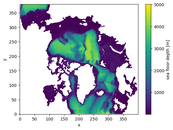
ds_bathy.depth.plot()
<matplotlib.collections.QuadMesh at 0x1550a6eb87d0>
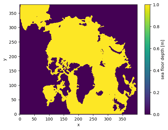
land_mask = ds_bathy.depth.isnull()
mask = 1 - land_mask
mask.plot()
<matplotlib.collections.QuadMesh at 0x1550a6f853d0>
Open a single archive snapshot#
open_dataset auto-detects the file type (archive, grid, bathymetry) from the
.b header. When grid= is provided, appropriate lon/lat coordinates are
attached to each variable based on its staggering point on the Arakawa C-grid.
ds = xhycom.open_dataset(DATA_PATH + "archm.2020_001_12", grid=GRID_PATH)
ds
<xarray.Dataset> Size: 3GB
Dimensions:     (time: 1, y: 380, x: 400, k: 50, ki: 51)
Coordinates:
  * time        (time) object 8B 2020-01-01 00:00:00
    lon         (y, x) float64 1MB -94.75 -94.58 -94.42 ... 99.09 98.95 98.82
    lat         (y, x) float64 1MB 39.06 39.16 39.26 39.36 ... 56.39 56.29 56.2
    lon_u       (y, x) float64 1MB -94.83 -94.67 -94.5 ... 99.16 99.02 98.89
    lat_u       (y, x) float64 1MB 39.01 39.11 39.21 39.31 ... 56.43 56.34 56.25
    lon_v       (y, x) float64 1MB -94.68 -94.52 -94.35 ... 99.0 98.87 98.74
    lat_v       (y, x) float64 1MB 38.99 39.09 39.19 39.29 ... 56.43 56.33 56.24
  * k           (k) int64 400B 1 2 3 4 5 6 7 8 9 ... 42 43 44 45 46 47 48 49 50
    dens        (k) float64 400B 0.1 0.2 0.3 0.4 0.5 ... 28.09 28.1 28.11 28.12
  * ki          (ki) int64 408B 0 1 2 3 4 5 6 7 8 ... 42 43 44 45 46 47 48 49 50
Dimensions without coordinates: y, x
Data variables: (12/83)
    montg1      (time, y, x) float64 1MB nan nan nan nan nan ... nan nan nan nan
    srfhgt      (time, y, x) float64 1MB nan nan nan nan nan ... nan nan nan nan
    oneta       (time, y, x) float64 1MB nan nan nan nan nan ... nan nan nan nan
    surflx      (time, y, x) float64 1MB nan nan nan nan nan ... nan nan nan nan
    wtrflx      (time, y, x) float64 1MB nan nan nan nan nan ... nan nan nan nan
    salflx      (time, y, x) float64 1MB nan nan nan nan nan ... nan nan nan nan
    ...          ...
    CO2_wind    (time, y, x) float64 1MB nan nan nan nan nan ... nan nan nan nan
    ECO_bots    (time, y, x) float64 1MB nan nan nan nan nan ... nan nan nan nan
    surface__1  (time, y, x) float64 1MB nan nan nan nan nan ... nan nan nan nan
    surface__2  (time, y, x) float64 1MB nan nan nan nan nan ... nan nan nan nan
    si_u        (time, y, x) float64 1MB nan nan nan nan nan ... nan nan nan nan
    si_v        (time, y, x) float64 1MB nan nan nan nan nan ... nan nan nan nan
Attributes:
    iversn:   23
    iexpt:    28
yrflag: 3- time: 1
- y: 380
- x: 400
- k: 50
- ki: 51
- time(time)object2020-01-01 00:00:00
- long_name :
- time
- axis :
- T
array([cftime.DatetimeGregorian(2020, 1, 1, 0, 0, 0, 0, has_year_zero=False)], dtype=object) - lon(y, x)float64-94.75 -94.58 ... 98.95 98.82
- long_name :
- longitude (T-point)
- units :
- degrees_east
- standard_name :
- longitude
array([[ -94.74750519, -94.58249664, -94.41687775, ..., 5.86695623, 6.06488323, 6.26205826], [ -94.87778473, -94.71282959, -94.5472641 , ..., 5.99605846, 6.1941061 , 6.391397 ], [ -95.00868225, -94.84378815, -94.67826843, ..., 6.12591982, 6.32408571, 6.5214901 ], ..., [-173.207901 , -173.30162048, -173.39605713, ..., 98.75035858, 98.61607361, 98.48277283], [-173.36988831, -173.46382141, -173.55848694, ..., 98.92017365, 98.78582764, 98.65245819], [-173.53115845, -173.62532043, -173.72019958, ..., 99.08900452, 98.95459747, 98.82115936]], shape=(380, 400)) - lat(y, x)float6439.06 39.16 39.26 ... 56.29 56.2
- long_name :
- latitude (T-point)
- units :
- degrees_north
- standard_name :
- latitude
array([[39.05597305, 39.15685272, 39.25762558, ..., 43.83851242, 43.74554825, 43.65235138], [39.18373108, 39.28490067, 39.38597107, ..., 43.98142242, 43.888134 , 43.79462051], [39.31121063, 39.41267776, 39.51403809, ..., 44.12407684, 44.03046799, 43.93662643], ..., [51.74200058, 51.84247589, 51.94287109, ..., 56.53710175, 56.44309616, 56.34889603], [51.68408203, 51.78424835, 51.88433075, ..., 56.46269226, 56.36904907, 56.27520752], [51.62594986, 51.72580338, 51.82557678, ..., 56.3881073 , 56.29482269, 56.20133972]], shape=(380, 400)) - lon_u(y, x)float64-94.83 -94.67 -94.5 ... 99.02 98.89
- long_name :
- longitude (U-point)
- units :
- degrees_east
array([[ -94.82977295, -94.66507721, -94.49976349, ..., 5.76771021, 5.96601391, 6.16356468], [ -94.9600296 , -94.79538727, -94.63012695, ..., 5.89674997, 6.09517717, 6.2928462 ], [ -95.09089661, -94.92630768, -94.7611084 , ..., 6.02655029, 6.22509813, 6.42288303], ..., [-173.16131592, -173.25466919, -173.34875488, ..., 98.81787109, 98.68309021, 98.54930115], [-173.32318115, -173.41676331, -173.51106262, ..., 98.98771667, 98.85287476, 98.71901703], [-173.48432922, -173.57815552, -173.67266846, ..., 99.15657806, 99.02167511, 98.88775635]], shape=(380, 400)) - lat_u(y, x)float6439.01 39.11 39.21 ... 56.34 56.25
- long_name :
- latitude (U-point)
- units :
- degrees_north
array([[39.00549698, 39.10642624, 39.2072525 , ..., 43.88490677, 43.79206085, 43.69897842], [39.13310623, 39.23432922, 39.33544922, ..., 44.02797699, 43.93480682, 43.84140778], [39.26044464, 39.36195755, 39.46337128, ..., 44.17079163, 44.07730103, 43.98357391], ..., [51.69173431, 51.79224777, 51.89268494, ..., 56.58403015, 56.49012375, 56.39601898], [51.63396835, 51.73417664, 51.83430099, ..., 56.50944138, 56.41589737, 56.32215118], [51.57598877, 51.67588806, 51.77569962, ..., 56.43467712, 56.3414917 , 56.24810791]], shape=(380, 400)) - lon_v(y, x)float64-94.68 -94.52 ... 98.87 98.74
- long_name :
- longitude (V-point)
- units :
- degrees_east
array([[ -94.6825943 , -94.51755524, -94.35191345, ..., 5.8026886 , 6.00055408, 6.19766998], [ -94.81256866, -94.64758301, -94.481987 , ..., 5.9314127 , 6.12940025, 6.32663393], [ -94.94315338, -94.77822876, -94.61268616, ..., 6.06089401, 6.25900126, 6.4563489 ], ..., [-173.12664795, -173.22024536, -173.3145752 , ..., 98.66507721, 98.53083038, 98.39756775], [-173.28898621, -173.3828125 , -173.47735596, ..., 98.83538818, 98.70107269, 98.56773376], [-173.4506073 , -173.54466248, -173.63943481, ..., 99.00471497, 98.87033081, 98.73693085]], shape=(380, 400)) - lat_v(y, x)float6438.99 39.09 39.19 ... 56.33 56.24
- long_name :
- latitude (V-point)
- units :
- degrees_north
array([[38.99199295, 39.09272385, 39.19335175, ..., 43.76696396, 43.67416 , 43.58112335], [39.11988831, 39.22091293, 39.32183075, ..., 43.90999985, 43.81687546, 43.72351837], [39.24750519, 39.34882355, 39.45003891, ..., 44.05278015, 43.95933151, 43.86565399], ..., [51.77088165, 51.87150955, 51.97205734, ..., 56.57423782, 56.48004913, 56.38566971], [51.71306992, 51.81338882, 51.91362762, ..., 56.49991989, 56.4060936 , 56.31207275], [51.65504074, 51.75505447, 51.85498047, ..., 56.42542267, 56.33195877, 56.23829651]], shape=(380, 400)) - k(k)int641 2 3 4 5 6 7 ... 45 46 47 48 49 50
- long_name :
- layer index
- units :
- 1
- axis :
- Z
array([ 1, 2, 3, 4, 5, 6, 7, 8, 9, 10, 11, 12, 13, 14, 15, 16, 17, 18, 19, 20, 21, 22, 23, 24, 25, 26, 27, 28, 29, 30, 31, 32, 33, 34, 35, 36, 37, 38, 39, 40, 41, 42, 43, 44, 45, 46, 47, 48, 49, 50]) - dens(k)float640.1 0.2 0.3 ... 28.1 28.11 28.12
- long_name :
- target sigma-2 layer density
- units :
- kg m-3
array([ 0.1 , 0.2 , 0.3 , 0.4 , 0.5 , 0.6 , 0.7 , 0.8 , 0.9 , 1. , 24.05, 25.72, 26.4 , 26.9 , 27.13, 27.19, 27.25, 27.29, 27.34, 27.42, 27.5 , 27.56, 27.63, 27.66, 27.69, 27.72, 27.74, 27.76, 27.78, 27.8 , 27.82, 27.85, 27.87, 27.9 , 27.93, 27.95, 27.97, 27.99, 28.01, 28.02, 28.03, 28.04, 28.05, 28.06, 28.07, 28.08, 28.09, 28.1 , 28.11, 28.12]) - ki(ki)int640 1 2 3 4 5 6 ... 45 46 47 48 49 50
- long_name :
- layer interface index
- units :
- 1
- axis :
- Z
array([ 0,  1,  2,  3,  4,  5,  6,  7,  8,  9, 10, 11, 12, 13, 14, 15, 16, 17,
       18, 19, 20, 21, 22, 23, 24, 25, 26, 27, 28, 29, 30, 31, 32, 33, 34, 35,
       36, 37, 38, 39, 40, 41, 42, 43, 44, 45, 46, 47, 48, 49, 50])
- montg1(time, y, x)float64nan nan nan nan ... nan nan nan nan
- long_name :
- Montgomery potential
- units :
- m2 s-2
array([[[nan, nan, nan, ..., nan, nan, nan], [nan, nan, nan, ..., nan, nan, nan], [nan, nan, nan, ..., nan, nan, nan], ..., [nan, nan, nan, ..., nan, nan, nan], [nan, nan, nan, ..., nan, nan, nan], [nan, nan, nan, ..., nan, nan, nan]]], shape=(1, 380, 400)) - srfhgt(time, y, x)float64nan nan nan nan ... nan nan nan nan
- long_name :
- sea surface height
- units :
- Pa
array([[[nan, nan, nan, ..., nan, nan, nan], [nan, nan, nan, ..., nan, nan, nan], [nan, nan, nan, ..., nan, nan, nan], ..., [nan, nan, nan, ..., nan, nan, nan], [nan, nan, nan, ..., nan, nan, nan], [nan, nan, nan, ..., nan, nan, nan]]], shape=(1, 380, 400)) - oneta(time, y, x)float64nan nan nan nan ... nan nan nan nan
- long_name :
- free surface elevation
- units :
- m
array([[[nan, nan, nan, ..., nan, nan, nan], [nan, nan, nan, ..., nan, nan, nan], [nan, nan, nan, ..., nan, nan, nan], ..., [nan, nan, nan, ..., nan, nan, nan], [nan, nan, nan, ..., nan, nan, nan], [nan, nan, nan, ..., nan, nan, nan]]], shape=(1, 380, 400)) - surflx(time, y, x)float64nan nan nan nan ... nan nan nan nan
- long_name :
- net surface heat flux
- units :
- W m-2
array([[[nan, nan, nan, ..., nan, nan, nan], [nan, nan, nan, ..., nan, nan, nan], [nan, nan, nan, ..., nan, nan, nan], ..., [nan, nan, nan, ..., nan, nan, nan], [nan, nan, nan, ..., nan, nan, nan], [nan, nan, nan, ..., nan, nan, nan]]], shape=(1, 380, 400)) - wtrflx(time, y, x)float64nan nan nan nan ... nan nan nan nan
- long_name :
- net surface freshwater flux
- units :
- m s-1
array([[[nan, nan, nan, ..., nan, nan, nan], [nan, nan, nan, ..., nan, nan, nan], [nan, nan, nan, ..., nan, nan, nan], ..., [nan, nan, nan, ..., nan, nan, nan], [nan, nan, nan, ..., nan, nan, nan], [nan, nan, nan, ..., nan, nan, nan]]], shape=(1, 380, 400)) - salflx(time, y, x)float64nan nan nan nan ... nan nan nan nan
- long_name :
- surface salt flux
- units :
- PSU m s-1
array([[[nan, nan, nan, ..., nan, nan, nan], [nan, nan, nan, ..., nan, nan, nan], [nan, nan, nan, ..., nan, nan, nan], ..., [nan, nan, nan, ..., nan, nan, nan], [nan, nan, nan, ..., nan, nan, nan], [nan, nan, nan, ..., nan, nan, nan]]], shape=(1, 380, 400)) - bl_dpth(time, y, x)float64nan nan nan nan ... nan nan nan nan
- long_name :
- boundary layer depth
- units :
- Pa
array([[[nan, nan, nan, ..., nan, nan, nan], [nan, nan, nan, ..., nan, nan, nan], [nan, nan, nan, ..., nan, nan, nan], ..., [nan, nan, nan, ..., nan, nan, nan], [nan, nan, nan, ..., nan, nan, nan], [nan, nan, nan, ..., nan, nan, nan]]], shape=(1, 380, 400)) - mix_dpth(time, y, x)float64nan nan nan nan ... nan nan nan nan
- long_name :
- mixed layer depth
- units :
- Pa
array([[[nan, nan, nan, ..., nan, nan, nan], [nan, nan, nan, ..., nan, nan, nan], [nan, nan, nan, ..., nan, nan, nan], ..., [nan, nan, nan, ..., nan, nan, nan], [nan, nan, nan, ..., nan, nan, nan], [nan, nan, nan, ..., nan, nan, nan]]], shape=(1, 380, 400)) - tmix(time, y, x)float64nan nan nan nan ... nan nan nan nan
- long_name :
- mixed layer temperature
- units :
- degC
array([[[nan, nan, nan, ..., nan, nan, nan], [nan, nan, nan, ..., nan, nan, nan], [nan, nan, nan, ..., nan, nan, nan], ..., [nan, nan, nan, ..., nan, nan, nan], [nan, nan, nan, ..., nan, nan, nan], [nan, nan, nan, ..., nan, nan, nan]]], shape=(1, 380, 400)) - smix(time, y, x)float64nan nan nan nan ... nan nan nan nan
- long_name :
- mixed layer salinity
- units :
- PSU
array([[[nan, nan, nan, ..., nan, nan, nan], [nan, nan, nan, ..., nan, nan, nan], [nan, nan, nan, ..., nan, nan, nan], ..., [nan, nan, nan, ..., nan, nan, nan], [nan, nan, nan, ..., nan, nan, nan], [nan, nan, nan, ..., nan, nan, nan]]], shape=(1, 380, 400)) - thmix(time, y, x)float64nan nan nan nan ... nan nan nan nan
- long_name :
- mixed layer thickness
- units :
- Pa
array([[[nan, nan, nan, ..., nan, nan, nan], [nan, nan, nan, ..., nan, nan, nan], [nan, nan, nan, ..., nan, nan, nan], ..., [nan, nan, nan, ..., nan, nan, nan], [nan, nan, nan, ..., nan, nan, nan], [nan, nan, nan, ..., nan, nan, nan]]], shape=(1, 380, 400)) - umix(time, y, x)float64nan nan nan nan ... nan nan nan nan
- long_name :
- mixed layer x velocity
- units :
- m s-1
array([[[nan, nan, nan, ..., nan, nan, nan], [nan, nan, nan, ..., nan, nan, nan], [nan, nan, nan, ..., nan, nan, nan], ..., [nan, nan, nan, ..., nan, nan, nan], [nan, nan, nan, ..., nan, nan, nan], [nan, nan, nan, ..., nan, nan, nan]]], shape=(1, 380, 400)) - vmix(time, y, x)float64nan nan nan nan ... nan nan nan nan
- long_name :
- mixed layer y velocity
- units :
- m s-1
array([[[nan, nan, nan, ..., nan, nan, nan], [nan, nan, nan, ..., nan, nan, nan], [nan, nan, nan, ..., nan, nan, nan], ..., [nan, nan, nan, ..., nan, nan, nan], [nan, nan, nan, ..., nan, nan, nan], [nan, nan, nan, ..., nan, nan, nan]]], shape=(1, 380, 400)) - kemix(time, y, x)float64nan nan nan nan ... nan nan nan nan
- long_name :
- mixed layer kinetic energy
- units :
- m2 s-2
array([[[nan, nan, nan, ..., nan, nan, nan], [nan, nan, nan, ..., nan, nan, nan], [nan, nan, nan, ..., nan, nan, nan], ..., [nan, nan, nan, ..., nan, nan, nan], [nan, nan, nan, ..., nan, nan, nan], [nan, nan, nan, ..., nan, nan, nan]]], shape=(1, 380, 400)) - covice(time, y, x)float64nan nan nan nan ... nan nan nan nan
- long_name :
- sea ice coverage fraction
- units :
- 1
array([[[nan, nan, nan, ..., nan, nan, nan], [nan, nan, nan, ..., nan, nan, nan], [nan, nan, nan, ..., nan, nan, nan], ..., [nan, nan, nan, ..., nan, nan, nan], [nan, nan, nan, ..., nan, nan, nan], [nan, nan, nan, ..., nan, nan, nan]]], shape=(1, 380, 400)) - thkice(time, y, x)float64nan nan nan nan ... nan nan nan nan
- long_name :
- sea ice thickness
- units :
- m
array([[[nan, nan, nan, ..., nan, nan, nan], [nan, nan, nan, ..., nan, nan, nan], [nan, nan, nan, ..., nan, nan, nan], ..., [nan, nan, nan, ..., nan, nan, nan], [nan, nan, nan, ..., nan, nan, nan], [nan, nan, nan, ..., nan, nan, nan]]], shape=(1, 380, 400)) - temice(time, y, x)float64nan nan nan nan ... nan nan nan nan
- long_name :
- sea ice surface temperature
- units :
- degC
array([[[nan, nan, nan, ..., nan, nan, nan], [nan, nan, nan, ..., nan, nan, nan], [nan, nan, nan, ..., nan, nan, nan], ..., [nan, nan, nan, ..., nan, nan, nan], [nan, nan, nan, ..., nan, nan, nan], [nan, nan, nan, ..., nan, nan, nan]]], shape=(1, 380, 400)) - u_btrop(time, y, x)float64nan nan nan nan ... nan nan nan nan
- long_name :
- barotropic x velocity
- units :
- m s-1
array([[[nan, nan, nan, ..., nan, nan, nan], [nan, nan, nan, ..., nan, nan, nan], [nan, nan, nan, ..., nan, nan, nan], ..., [nan, nan, nan, ..., nan, nan, nan], [nan, nan, nan, ..., nan, nan, nan], [nan, nan, nan, ..., nan, nan, nan]]], shape=(1, 380, 400)) - v_btrop(time, y, x)float64nan nan nan nan ... nan nan nan nan
- long_name :
- barotropic y velocity
- units :
- m s-1
array([[[nan, nan, nan, ..., nan, nan, nan], [nan, nan, nan, ..., nan, nan, nan], [nan, nan, nan, ..., nan, nan, nan], ..., [nan, nan, nan, ..., nan, nan, nan], [nan, nan, nan, ..., nan, nan, nan], [nan, nan, nan, ..., nan, nan, nan]]], shape=(1, 380, 400)) - kebtrop(time, y, x)float64nan nan nan nan ... nan nan nan nan
- long_name :
- barotropic kinetic energy
- units :
- m2 s-2
array([[[nan, nan, nan, ..., nan, nan, nan], [nan, nan, nan, ..., nan, nan, nan], [nan, nan, nan, ..., nan, nan, nan], ..., [nan, nan, nan, ..., nan, nan, nan], [nan, nan, nan, ..., nan, nan, nan], [nan, nan, nan, ..., nan, nan, nan]]], shape=(1, 380, 400)) - u-vel.(time, k, y, x)float64nan nan nan nan ... nan nan nan nan
- long_name :
- sea water x velocity
- units :
- m s-1
array([[[[nan, nan, nan, ..., nan, nan, nan], [nan, nan, nan, ..., nan, nan, nan], [nan, nan, nan, ..., nan, nan, nan], ..., [nan, nan, nan, ..., nan, nan, nan], [nan, nan, nan, ..., nan, nan, nan], [nan, nan, nan, ..., nan, nan, nan]], [[nan, nan, nan, ..., nan, nan, nan], [nan, nan, nan, ..., nan, nan, nan], [nan, nan, nan, ..., nan, nan, nan], ..., [nan, nan, nan, ..., nan, nan, nan], [nan, nan, nan, ..., nan, nan, nan], [nan, nan, nan, ..., nan, nan, nan]], [[nan, nan, nan, ..., nan, nan, nan], [nan, nan, nan, ..., nan, nan, nan], [nan, nan, nan, ..., nan, nan, nan], ..., ... ..., [nan, nan, nan, ..., nan, nan, nan], [nan, nan, nan, ..., nan, nan, nan], [nan, nan, nan, ..., nan, nan, nan]], [[nan, nan, nan, ..., nan, nan, nan], [nan, nan, nan, ..., nan, nan, nan], [nan, nan, nan, ..., nan, nan, nan], ..., [nan, nan, nan, ..., nan, nan, nan], [nan, nan, nan, ..., nan, nan, nan], [nan, nan, nan, ..., nan, nan, nan]], [[nan, nan, nan, ..., nan, nan, nan], [nan, nan, nan, ..., nan, nan, nan], [nan, nan, nan, ..., nan, nan, nan], ..., [nan, nan, nan, ..., nan, nan, nan], [nan, nan, nan, ..., nan, nan, nan], [nan, nan, nan, ..., nan, nan, nan]]]], shape=(1, 50, 380, 400)) - v-vel.(time, k, y, x)float64nan nan nan nan ... nan nan nan nan
- long_name :
- sea water y velocity
- units :
- m s-1
array([[[[nan, nan, nan, ..., nan, nan, nan], [nan, nan, nan, ..., nan, nan, nan], [nan, nan, nan, ..., nan, nan, nan], ..., [nan, nan, nan, ..., nan, nan, nan], [nan, nan, nan, ..., nan, nan, nan], [nan, nan, nan, ..., nan, nan, nan]], [[nan, nan, nan, ..., nan, nan, nan], [nan, nan, nan, ..., nan, nan, nan], [nan, nan, nan, ..., nan, nan, nan], ..., [nan, nan, nan, ..., nan, nan, nan], [nan, nan, nan, ..., nan, nan, nan], [nan, nan, nan, ..., nan, nan, nan]], [[nan, nan, nan, ..., nan, nan, nan], [nan, nan, nan, ..., nan, nan, nan], [nan, nan, nan, ..., nan, nan, nan], ..., ... ..., [nan, nan, nan, ..., nan, nan, nan], [nan, nan, nan, ..., nan, nan, nan], [nan, nan, nan, ..., nan, nan, nan]], [[nan, nan, nan, ..., nan, nan, nan], [nan, nan, nan, ..., nan, nan, nan], [nan, nan, nan, ..., nan, nan, nan], ..., [nan, nan, nan, ..., nan, nan, nan], [nan, nan, nan, ..., nan, nan, nan], [nan, nan, nan, ..., nan, nan, nan]], [[nan, nan, nan, ..., nan, nan, nan], [nan, nan, nan, ..., nan, nan, nan], [nan, nan, nan, ..., nan, nan, nan], ..., [nan, nan, nan, ..., nan, nan, nan], [nan, nan, nan, ..., nan, nan, nan], [nan, nan, nan, ..., nan, nan, nan]]]], shape=(1, 50, 380, 400)) - k.e.(time, k, y, x)float64nan nan nan nan ... nan nan nan nan
- long_name :
- kinetic energy
- units :
- m2 s-2
array([[[[nan, nan, nan, ..., nan, nan, nan], [nan, nan, nan, ..., nan, nan, nan], [nan, nan, nan, ..., nan, nan, nan], ..., [nan, nan, nan, ..., nan, nan, nan], [nan, nan, nan, ..., nan, nan, nan], [nan, nan, nan, ..., nan, nan, nan]], [[nan, nan, nan, ..., nan, nan, nan], [nan, nan, nan, ..., nan, nan, nan], [nan, nan, nan, ..., nan, nan, nan], ..., [nan, nan, nan, ..., nan, nan, nan], [nan, nan, nan, ..., nan, nan, nan], [nan, nan, nan, ..., nan, nan, nan]], [[nan, nan, nan, ..., nan, nan, nan], [nan, nan, nan, ..., nan, nan, nan], [nan, nan, nan, ..., nan, nan, nan], ..., ... ..., [nan, nan, nan, ..., nan, nan, nan], [nan, nan, nan, ..., nan, nan, nan], [nan, nan, nan, ..., nan, nan, nan]], [[nan, nan, nan, ..., nan, nan, nan], [nan, nan, nan, ..., nan, nan, nan], [nan, nan, nan, ..., nan, nan, nan], ..., [nan, nan, nan, ..., nan, nan, nan], [nan, nan, nan, ..., nan, nan, nan], [nan, nan, nan, ..., nan, nan, nan]], [[nan, nan, nan, ..., nan, nan, nan], [nan, nan, nan, ..., nan, nan, nan], [nan, nan, nan, ..., nan, nan, nan], ..., [nan, nan, nan, ..., nan, nan, nan], [nan, nan, nan, ..., nan, nan, nan], [nan, nan, nan, ..., nan, nan, nan]]]], shape=(1, 50, 380, 400)) - thknss(time, k, y, x)float64nan nan nan nan ... nan nan nan nan
- long_name :
- layer pressure thickness
- units :
- Pa
array([[[[nan, nan, nan, ..., nan, nan, nan], [nan, nan, nan, ..., nan, nan, nan], [nan, nan, nan, ..., nan, nan, nan], ..., [nan, nan, nan, ..., nan, nan, nan], [nan, nan, nan, ..., nan, nan, nan], [nan, nan, nan, ..., nan, nan, nan]], [[nan, nan, nan, ..., nan, nan, nan], [nan, nan, nan, ..., nan, nan, nan], [nan, nan, nan, ..., nan, nan, nan], ..., [nan, nan, nan, ..., nan, nan, nan], [nan, nan, nan, ..., nan, nan, nan], [nan, nan, nan, ..., nan, nan, nan]], [[nan, nan, nan, ..., nan, nan, nan], [nan, nan, nan, ..., nan, nan, nan], [nan, nan, nan, ..., nan, nan, nan], ..., ... ..., [nan, nan, nan, ..., nan, nan, nan], [nan, nan, nan, ..., nan, nan, nan], [nan, nan, nan, ..., nan, nan, nan]], [[nan, nan, nan, ..., nan, nan, nan], [nan, nan, nan, ..., nan, nan, nan], [nan, nan, nan, ..., nan, nan, nan], ..., [nan, nan, nan, ..., nan, nan, nan], [nan, nan, nan, ..., nan, nan, nan], [nan, nan, nan, ..., nan, nan, nan]], [[nan, nan, nan, ..., nan, nan, nan], [nan, nan, nan, ..., nan, nan, nan], [nan, nan, nan, ..., nan, nan, nan], ..., [nan, nan, nan, ..., nan, nan, nan], [nan, nan, nan, ..., nan, nan, nan], [nan, nan, nan, ..., nan, nan, nan]]]], shape=(1, 50, 380, 400)) - temp(time, k, y, x)float64nan nan nan nan ... nan nan nan nan
- long_name :
- sea water potential temperature
- units :
- degC
array([[[[nan, nan, nan, ..., nan, nan, nan], [nan, nan, nan, ..., nan, nan, nan], [nan, nan, nan, ..., nan, nan, nan], ..., [nan, nan, nan, ..., nan, nan, nan], [nan, nan, nan, ..., nan, nan, nan], [nan, nan, nan, ..., nan, nan, nan]], [[nan, nan, nan, ..., nan, nan, nan], [nan, nan, nan, ..., nan, nan, nan], [nan, nan, nan, ..., nan, nan, nan], ..., [nan, nan, nan, ..., nan, nan, nan], [nan, nan, nan, ..., nan, nan, nan], [nan, nan, nan, ..., nan, nan, nan]], [[nan, nan, nan, ..., nan, nan, nan], [nan, nan, nan, ..., nan, nan, nan], [nan, nan, nan, ..., nan, nan, nan], ..., ... ..., [nan, nan, nan, ..., nan, nan, nan], [nan, nan, nan, ..., nan, nan, nan], [nan, nan, nan, ..., nan, nan, nan]], [[nan, nan, nan, ..., nan, nan, nan], [nan, nan, nan, ..., nan, nan, nan], [nan, nan, nan, ..., nan, nan, nan], ..., [nan, nan, nan, ..., nan, nan, nan], [nan, nan, nan, ..., nan, nan, nan], [nan, nan, nan, ..., nan, nan, nan]], [[nan, nan, nan, ..., nan, nan, nan], [nan, nan, nan, ..., nan, nan, nan], [nan, nan, nan, ..., nan, nan, nan], ..., [nan, nan, nan, ..., nan, nan, nan], [nan, nan, nan, ..., nan, nan, nan], [nan, nan, nan, ..., nan, nan, nan]]]], shape=(1, 50, 380, 400)) - salin(time, k, y, x)float64nan nan nan nan ... nan nan nan nan
- long_name :
- sea water salinity
- units :
- PSU
array([[[[nan, nan, nan, ..., nan, nan, nan], [nan, nan, nan, ..., nan, nan, nan], [nan, nan, nan, ..., nan, nan, nan], ..., [nan, nan, nan, ..., nan, nan, nan], [nan, nan, nan, ..., nan, nan, nan], [nan, nan, nan, ..., nan, nan, nan]], [[nan, nan, nan, ..., nan, nan, nan], [nan, nan, nan, ..., nan, nan, nan], [nan, nan, nan, ..., nan, nan, nan], ..., [nan, nan, nan, ..., nan, nan, nan], [nan, nan, nan, ..., nan, nan, nan], [nan, nan, nan, ..., nan, nan, nan]], [[nan, nan, nan, ..., nan, nan, nan], [nan, nan, nan, ..., nan, nan, nan], [nan, nan, nan, ..., nan, nan, nan], ..., ... ..., [nan, nan, nan, ..., nan, nan, nan], [nan, nan, nan, ..., nan, nan, nan], [nan, nan, nan, ..., nan, nan, nan]], [[nan, nan, nan, ..., nan, nan, nan], [nan, nan, nan, ..., nan, nan, nan], [nan, nan, nan, ..., nan, nan, nan], ..., [nan, nan, nan, ..., nan, nan, nan], [nan, nan, nan, ..., nan, nan, nan], [nan, nan, nan, ..., nan, nan, nan]], [[nan, nan, nan, ..., nan, nan, nan], [nan, nan, nan, ..., nan, nan, nan], [nan, nan, nan, ..., nan, nan, nan], ..., [nan, nan, nan, ..., nan, nan, nan], [nan, nan, nan, ..., nan, nan, nan], [nan, nan, nan, ..., nan, nan, nan]]]], shape=(1, 50, 380, 400)) - density(time, k, y, x)float64nan nan nan nan ... nan nan nan nan
- long_name :
- sea water potential density (sigma-2)
- units :
- kg m-3
array([[[[nan, nan, nan, ..., nan, nan, nan], [nan, nan, nan, ..., nan, nan, nan], [nan, nan, nan, ..., nan, nan, nan], ..., [nan, nan, nan, ..., nan, nan, nan], [nan, nan, nan, ..., nan, nan, nan], [nan, nan, nan, ..., nan, nan, nan]], [[nan, nan, nan, ..., nan, nan, nan], [nan, nan, nan, ..., nan, nan, nan], [nan, nan, nan, ..., nan, nan, nan], ..., [nan, nan, nan, ..., nan, nan, nan], [nan, nan, nan, ..., nan, nan, nan], [nan, nan, nan, ..., nan, nan, nan]], [[nan, nan, nan, ..., nan, nan, nan], [nan, nan, nan, ..., nan, nan, nan], [nan, nan, nan, ..., nan, nan, nan], ..., ... ..., [nan, nan, nan, ..., nan, nan, nan], [nan, nan, nan, ..., nan, nan, nan], [nan, nan, nan, ..., nan, nan, nan]], [[nan, nan, nan, ..., nan, nan, nan], [nan, nan, nan, ..., nan, nan, nan], [nan, nan, nan, ..., nan, nan, nan], ..., [nan, nan, nan, ..., nan, nan, nan], [nan, nan, nan, ..., nan, nan, nan], [nan, nan, nan, ..., nan, nan, nan]], [[nan, nan, nan, ..., nan, nan, nan], [nan, nan, nan, ..., nan, nan, nan], [nan, nan, nan, ..., nan, nan, nan], ..., [nan, nan, nan, ..., nan, nan, nan], [nan, nan, nan, ..., nan, nan, nan], [nan, nan, nan, ..., nan, nan, nan]]]], shape=(1, 50, 380, 400)) - CO2_c(time, k, y, x)float64nan nan nan nan ... nan nan nan nan
- long_name :
- dissolved inorganic carbon
- units :
- mmol C m-3
array([[[[nan, nan, nan, ..., nan, nan, nan], [nan, nan, nan, ..., nan, nan, nan], [nan, nan, nan, ..., nan, nan, nan], ..., [nan, nan, nan, ..., nan, nan, nan], [nan, nan, nan, ..., nan, nan, nan], [nan, nan, nan, ..., nan, nan, nan]], [[nan, nan, nan, ..., nan, nan, nan], [nan, nan, nan, ..., nan, nan, nan], [nan, nan, nan, ..., nan, nan, nan], ..., [nan, nan, nan, ..., nan, nan, nan], [nan, nan, nan, ..., nan, nan, nan], [nan, nan, nan, ..., nan, nan, nan]], [[nan, nan, nan, ..., nan, nan, nan], [nan, nan, nan, ..., nan, nan, nan], [nan, nan, nan, ..., nan, nan, nan], ..., ... ..., [nan, nan, nan, ..., nan, nan, nan], [nan, nan, nan, ..., nan, nan, nan], [nan, nan, nan, ..., nan, nan, nan]], [[nan, nan, nan, ..., nan, nan, nan], [nan, nan, nan, ..., nan, nan, nan], [nan, nan, nan, ..., nan, nan, nan], ..., [nan, nan, nan, ..., nan, nan, nan], [nan, nan, nan, ..., nan, nan, nan], [nan, nan, nan, ..., nan, nan, nan]], [[nan, nan, nan, ..., nan, nan, nan], [nan, nan, nan, ..., nan, nan, nan], [nan, nan, nan, ..., nan, nan, nan], ..., [nan, nan, nan, ..., nan, nan, nan], [nan, nan, nan, ..., nan, nan, nan], [nan, nan, nan, ..., nan, nan, nan]]]], shape=(1, 50, 380, 400)) - CO2_TA(time, k, y, x)float64nan nan nan nan ... nan nan nan nan
- long_name :
- total alkalinity
- units :
- mmol eq m-3
array([[[[nan, nan, nan, ..., nan, nan, nan], [nan, nan, nan, ..., nan, nan, nan], [nan, nan, nan, ..., nan, nan, nan], ..., [nan, nan, nan, ..., nan, nan, nan], [nan, nan, nan, ..., nan, nan, nan], [nan, nan, nan, ..., nan, nan, nan]], [[nan, nan, nan, ..., nan, nan, nan], [nan, nan, nan, ..., nan, nan, nan], [nan, nan, nan, ..., nan, nan, nan], ..., [nan, nan, nan, ..., nan, nan, nan], [nan, nan, nan, ..., nan, nan, nan], [nan, nan, nan, ..., nan, nan, nan]], [[nan, nan, nan, ..., nan, nan, nan], [nan, nan, nan, ..., nan, nan, nan], [nan, nan, nan, ..., nan, nan, nan], ..., ... ..., [nan, nan, nan, ..., nan, nan, nan], [nan, nan, nan, ..., nan, nan, nan], [nan, nan, nan, ..., nan, nan, nan]], [[nan, nan, nan, ..., nan, nan, nan], [nan, nan, nan, ..., nan, nan, nan], [nan, nan, nan, ..., nan, nan, nan], ..., [nan, nan, nan, ..., nan, nan, nan], [nan, nan, nan, ..., nan, nan, nan], [nan, nan, nan, ..., nan, nan, nan]], [[nan, nan, nan, ..., nan, nan, nan], [nan, nan, nan, ..., nan, nan, nan], [nan, nan, nan, ..., nan, nan, nan], ..., [nan, nan, nan, ..., nan, nan, nan], [nan, nan, nan, ..., nan, nan, nan], [nan, nan, nan, ..., nan, nan, nan]]]], shape=(1, 50, 380, 400)) - ECO_no3(time, k, y, x)float64nan nan nan nan ... nan nan nan nan
- long_name :
- nitrate
- units :
- mmol N m-3
array([[[[nan, nan, nan, ..., nan, nan, nan], [nan, nan, nan, ..., nan, nan, nan], [nan, nan, nan, ..., nan, nan, nan], ..., [nan, nan, nan, ..., nan, nan, nan], [nan, nan, nan, ..., nan, nan, nan], [nan, nan, nan, ..., nan, nan, nan]], [[nan, nan, nan, ..., nan, nan, nan], [nan, nan, nan, ..., nan, nan, nan], [nan, nan, nan, ..., nan, nan, nan], ..., [nan, nan, nan, ..., nan, nan, nan], [nan, nan, nan, ..., nan, nan, nan], [nan, nan, nan, ..., nan, nan, nan]], [[nan, nan, nan, ..., nan, nan, nan], [nan, nan, nan, ..., nan, nan, nan], [nan, nan, nan, ..., nan, nan, nan], ..., ... ..., [nan, nan, nan, ..., nan, nan, nan], [nan, nan, nan, ..., nan, nan, nan], [nan, nan, nan, ..., nan, nan, nan]], [[nan, nan, nan, ..., nan, nan, nan], [nan, nan, nan, ..., nan, nan, nan], [nan, nan, nan, ..., nan, nan, nan], ..., [nan, nan, nan, ..., nan, nan, nan], [nan, nan, nan, ..., nan, nan, nan], [nan, nan, nan, ..., nan, nan, nan]], [[nan, nan, nan, ..., nan, nan, nan], [nan, nan, nan, ..., nan, nan, nan], [nan, nan, nan, ..., nan, nan, nan], ..., [nan, nan, nan, ..., nan, nan, nan], [nan, nan, nan, ..., nan, nan, nan], [nan, nan, nan, ..., nan, nan, nan]]]], shape=(1, 50, 380, 400)) - ECO_nh4(time, k, y, x)float64nan nan nan nan ... nan nan nan nan
- long_name :
- ammonium
- units :
- mmol N m-3
array([[[[nan, nan, nan, ..., nan, nan, nan], [nan, nan, nan, ..., nan, nan, nan], [nan, nan, nan, ..., nan, nan, nan], ..., [nan, nan, nan, ..., nan, nan, nan], [nan, nan, nan, ..., nan, nan, nan], [nan, nan, nan, ..., nan, nan, nan]], [[nan, nan, nan, ..., nan, nan, nan], [nan, nan, nan, ..., nan, nan, nan], [nan, nan, nan, ..., nan, nan, nan], ..., [nan, nan, nan, ..., nan, nan, nan], [nan, nan, nan, ..., nan, nan, nan], [nan, nan, nan, ..., nan, nan, nan]], [[nan, nan, nan, ..., nan, nan, nan], [nan, nan, nan, ..., nan, nan, nan], [nan, nan, nan, ..., nan, nan, nan], ..., ... ..., [nan, nan, nan, ..., nan, nan, nan], [nan, nan, nan, ..., nan, nan, nan], [nan, nan, nan, ..., nan, nan, nan]], [[nan, nan, nan, ..., nan, nan, nan], [nan, nan, nan, ..., nan, nan, nan], [nan, nan, nan, ..., nan, nan, nan], ..., [nan, nan, nan, ..., nan, nan, nan], [nan, nan, nan, ..., nan, nan, nan], [nan, nan, nan, ..., nan, nan, nan]], [[nan, nan, nan, ..., nan, nan, nan], [nan, nan, nan, ..., nan, nan, nan], [nan, nan, nan, ..., nan, nan, nan], ..., [nan, nan, nan, ..., nan, nan, nan], [nan, nan, nan, ..., nan, nan, nan], [nan, nan, nan, ..., nan, nan, nan]]]], shape=(1, 50, 380, 400)) - ECO_pho(time, k, y, x)float64nan nan nan nan ... nan nan nan nan
- long_name :
- phosphate
- units :
- mmol P m-3
array([[[[nan, nan, nan, ..., nan, nan, nan], [nan, nan, nan, ..., nan, nan, nan], [nan, nan, nan, ..., nan, nan, nan], ..., [nan, nan, nan, ..., nan, nan, nan], [nan, nan, nan, ..., nan, nan, nan], [nan, nan, nan, ..., nan, nan, nan]], [[nan, nan, nan, ..., nan, nan, nan], [nan, nan, nan, ..., nan, nan, nan], [nan, nan, nan, ..., nan, nan, nan], ..., [nan, nan, nan, ..., nan, nan, nan], [nan, nan, nan, ..., nan, nan, nan], [nan, nan, nan, ..., nan, nan, nan]], [[nan, nan, nan, ..., nan, nan, nan], [nan, nan, nan, ..., nan, nan, nan], [nan, nan, nan, ..., nan, nan, nan], ..., ... ..., [nan, nan, nan, ..., nan, nan, nan], [nan, nan, nan, ..., nan, nan, nan], [nan, nan, nan, ..., nan, nan, nan]], [[nan, nan, nan, ..., nan, nan, nan], [nan, nan, nan, ..., nan, nan, nan], [nan, nan, nan, ..., nan, nan, nan], ..., [nan, nan, nan, ..., nan, nan, nan], [nan, nan, nan, ..., nan, nan, nan], [nan, nan, nan, ..., nan, nan, nan]], [[nan, nan, nan, ..., nan, nan, nan], [nan, nan, nan, ..., nan, nan, nan], [nan, nan, nan, ..., nan, nan, nan], ..., [nan, nan, nan, ..., nan, nan, nan], [nan, nan, nan, ..., nan, nan, nan], [nan, nan, nan, ..., nan, nan, nan]]]], shape=(1, 50, 380, 400)) - ECO_sil(time, k, y, x)float64nan nan nan nan ... nan nan nan nan
- long_name :
- silicate
- units :
- mmol Si m-3
array([[[[nan, nan, nan, ..., nan, nan, nan], [nan, nan, nan, ..., nan, nan, nan], [nan, nan, nan, ..., nan, nan, nan], ..., [nan, nan, nan, ..., nan, nan, nan], [nan, nan, nan, ..., nan, nan, nan], [nan, nan, nan, ..., nan, nan, nan]], [[nan, nan, nan, ..., nan, nan, nan], [nan, nan, nan, ..., nan, nan, nan], [nan, nan, nan, ..., nan, nan, nan], ..., [nan, nan, nan, ..., nan, nan, nan], [nan, nan, nan, ..., nan, nan, nan], [nan, nan, nan, ..., nan, nan, nan]], [[nan, nan, nan, ..., nan, nan, nan], [nan, nan, nan, ..., nan, nan, nan], [nan, nan, nan, ..., nan, nan, nan], ..., ... ..., [nan, nan, nan, ..., nan, nan, nan], [nan, nan, nan, ..., nan, nan, nan], [nan, nan, nan, ..., nan, nan, nan]], [[nan, nan, nan, ..., nan, nan, nan], [nan, nan, nan, ..., nan, nan, nan], [nan, nan, nan, ..., nan, nan, nan], ..., [nan, nan, nan, ..., nan, nan, nan], [nan, nan, nan, ..., nan, nan, nan], [nan, nan, nan, ..., nan, nan, nan]], [[nan, nan, nan, ..., nan, nan, nan], [nan, nan, nan, ..., nan, nan, nan], [nan, nan, nan, ..., nan, nan, nan], ..., [nan, nan, nan, ..., nan, nan, nan], [nan, nan, nan, ..., nan, nan, nan], [nan, nan, nan, ..., nan, nan, nan]]]], shape=(1, 50, 380, 400)) - ECO_oxy(time, k, y, x)float64nan nan nan nan ... nan nan nan nan
- long_name :
- dissolved oxygen
- units :
- mmol O m-3
array([[[[nan, nan, nan, ..., nan, nan, nan], [nan, nan, nan, ..., nan, nan, nan], [nan, nan, nan, ..., nan, nan, nan], ..., [nan, nan, nan, ..., nan, nan, nan], [nan, nan, nan, ..., nan, nan, nan], [nan, nan, nan, ..., nan, nan, nan]], [[nan, nan, nan, ..., nan, nan, nan], [nan, nan, nan, ..., nan, nan, nan], [nan, nan, nan, ..., nan, nan, nan], ..., [nan, nan, nan, ..., nan, nan, nan], [nan, nan, nan, ..., nan, nan, nan], [nan, nan, nan, ..., nan, nan, nan]], [[nan, nan, nan, ..., nan, nan, nan], [nan, nan, nan, ..., nan, nan, nan], [nan, nan, nan, ..., nan, nan, nan], ..., ... ..., [nan, nan, nan, ..., nan, nan, nan], [nan, nan, nan, ..., nan, nan, nan], [nan, nan, nan, ..., nan, nan, nan]], [[nan, nan, nan, ..., nan, nan, nan], [nan, nan, nan, ..., nan, nan, nan], [nan, nan, nan, ..., nan, nan, nan], ..., [nan, nan, nan, ..., nan, nan, nan], [nan, nan, nan, ..., nan, nan, nan], [nan, nan, nan, ..., nan, nan, nan]], [[nan, nan, nan, ..., nan, nan, nan], [nan, nan, nan, ..., nan, nan, nan], [nan, nan, nan, ..., nan, nan, nan], ..., [nan, nan, nan, ..., nan, nan, nan], [nan, nan, nan, ..., nan, nan, nan], [nan, nan, nan, ..., nan, nan, nan]]]], shape=(1, 50, 380, 400)) - ECO_fla(time, k, y, x)float64nan nan nan nan ... nan nan nan nan
- long_name :
- flagellate carbon
- units :
- mmol C m-3
array([[[[nan, nan, nan, ..., nan, nan, nan], [nan, nan, nan, ..., nan, nan, nan], [nan, nan, nan, ..., nan, nan, nan], ..., [nan, nan, nan, ..., nan, nan, nan], [nan, nan, nan, ..., nan, nan, nan], [nan, nan, nan, ..., nan, nan, nan]], [[nan, nan, nan, ..., nan, nan, nan], [nan, nan, nan, ..., nan, nan, nan], [nan, nan, nan, ..., nan, nan, nan], ..., [nan, nan, nan, ..., nan, nan, nan], [nan, nan, nan, ..., nan, nan, nan], [nan, nan, nan, ..., nan, nan, nan]], [[nan, nan, nan, ..., nan, nan, nan], [nan, nan, nan, ..., nan, nan, nan], [nan, nan, nan, ..., nan, nan, nan], ..., ... ..., [nan, nan, nan, ..., nan, nan, nan], [nan, nan, nan, ..., nan, nan, nan], [nan, nan, nan, ..., nan, nan, nan]], [[nan, nan, nan, ..., nan, nan, nan], [nan, nan, nan, ..., nan, nan, nan], [nan, nan, nan, ..., nan, nan, nan], ..., [nan, nan, nan, ..., nan, nan, nan], [nan, nan, nan, ..., nan, nan, nan], [nan, nan, nan, ..., nan, nan, nan]], [[nan, nan, nan, ..., nan, nan, nan], [nan, nan, nan, ..., nan, nan, nan], [nan, nan, nan, ..., nan, nan, nan], ..., [nan, nan, nan, ..., nan, nan, nan], [nan, nan, nan, ..., nan, nan, nan], [nan, nan, nan, ..., nan, nan, nan]]]], shape=(1, 50, 380, 400)) - ECO_dia(time, k, y, x)float64nan nan nan nan ... nan nan nan nan
- long_name :
- diatom carbon
- units :
- mmol C m-3
array([[[[nan, nan, nan, ..., nan, nan, nan], [nan, nan, nan, ..., nan, nan, nan], [nan, nan, nan, ..., nan, nan, nan], ..., [nan, nan, nan, ..., nan, nan, nan], [nan, nan, nan, ..., nan, nan, nan], [nan, nan, nan, ..., nan, nan, nan]], [[nan, nan, nan, ..., nan, nan, nan], [nan, nan, nan, ..., nan, nan, nan], [nan, nan, nan, ..., nan, nan, nan], ..., [nan, nan, nan, ..., nan, nan, nan], [nan, nan, nan, ..., nan, nan, nan], [nan, nan, nan, ..., nan, nan, nan]], [[nan, nan, nan, ..., nan, nan, nan], [nan, nan, nan, ..., nan, nan, nan], [nan, nan, nan, ..., nan, nan, nan], ..., ... ..., [nan, nan, nan, ..., nan, nan, nan], [nan, nan, nan, ..., nan, nan, nan], [nan, nan, nan, ..., nan, nan, nan]], [[nan, nan, nan, ..., nan, nan, nan], [nan, nan, nan, ..., nan, nan, nan], [nan, nan, nan, ..., nan, nan, nan], ..., [nan, nan, nan, ..., nan, nan, nan], [nan, nan, nan, ..., nan, nan, nan], [nan, nan, nan, ..., nan, nan, nan]], [[nan, nan, nan, ..., nan, nan, nan], [nan, nan, nan, ..., nan, nan, nan], [nan, nan, nan, ..., nan, nan, nan], ..., [nan, nan, nan, ..., nan, nan, nan], [nan, nan, nan, ..., nan, nan, nan], [nan, nan, nan, ..., nan, nan, nan]]]], shape=(1, 50, 380, 400)) - ECO_ccl(time, k, y, x)float64nan nan nan nan ... nan nan nan nan
- long_name :
- coccolithophore carbon
- units :
- mmol C m-3
array([[[[nan, nan, nan, ..., nan, nan, nan], [nan, nan, nan, ..., nan, nan, nan], [nan, nan, nan, ..., nan, nan, nan], ..., [nan, nan, nan, ..., nan, nan, nan], [nan, nan, nan, ..., nan, nan, nan], [nan, nan, nan, ..., nan, nan, nan]], [[nan, nan, nan, ..., nan, nan, nan], [nan, nan, nan, ..., nan, nan, nan], [nan, nan, nan, ..., nan, nan, nan], ..., [nan, nan, nan, ..., nan, nan, nan], [nan, nan, nan, ..., nan, nan, nan], [nan, nan, nan, ..., nan, nan, nan]], [[nan, nan, nan, ..., nan, nan, nan], [nan, nan, nan, ..., nan, nan, nan], [nan, nan, nan, ..., nan, nan, nan], ..., ... ..., [nan, nan, nan, ..., nan, nan, nan], [nan, nan, nan, ..., nan, nan, nan], [nan, nan, nan, ..., nan, nan, nan]], [[nan, nan, nan, ..., nan, nan, nan], [nan, nan, nan, ..., nan, nan, nan], [nan, nan, nan, ..., nan, nan, nan], ..., [nan, nan, nan, ..., nan, nan, nan], [nan, nan, nan, ..., nan, nan, nan], [nan, nan, nan, ..., nan, nan, nan]], [[nan, nan, nan, ..., nan, nan, nan], [nan, nan, nan, ..., nan, nan, nan], [nan, nan, nan, ..., nan, nan, nan], ..., [nan, nan, nan, ..., nan, nan, nan], [nan, nan, nan, ..., nan, nan, nan], [nan, nan, nan, ..., nan, nan, nan]]]], shape=(1, 50, 380, 400)) - ECO_cclc(time, k, y, x)float64nan nan nan nan ... nan nan nan nan
- long_name :
- coccolithophore calcite carbon
- units :
- mmol C m-3
array([[[[nan, nan, nan, ..., nan, nan, nan], [nan, nan, nan, ..., nan, nan, nan], [nan, nan, nan, ..., nan, nan, nan], ..., [nan, nan, nan, ..., nan, nan, nan], [nan, nan, nan, ..., nan, nan, nan], [nan, nan, nan, ..., nan, nan, nan]], [[nan, nan, nan, ..., nan, nan, nan], [nan, nan, nan, ..., nan, nan, nan], [nan, nan, nan, ..., nan, nan, nan], ..., [nan, nan, nan, ..., nan, nan, nan], [nan, nan, nan, ..., nan, nan, nan], [nan, nan, nan, ..., nan, nan, nan]], [[nan, nan, nan, ..., nan, nan, nan], [nan, nan, nan, ..., nan, nan, nan], [nan, nan, nan, ..., nan, nan, nan], ..., ... ..., [nan, nan, nan, ..., nan, nan, nan], [nan, nan, nan, ..., nan, nan, nan], [nan, nan, nan, ..., nan, nan, nan]], [[nan, nan, nan, ..., nan, nan, nan], [nan, nan, nan, ..., nan, nan, nan], [nan, nan, nan, ..., nan, nan, nan], ..., [nan, nan, nan, ..., nan, nan, nan], [nan, nan, nan, ..., nan, nan, nan], [nan, nan, nan, ..., nan, nan, nan]], [[nan, nan, nan, ..., nan, nan, nan], [nan, nan, nan, ..., nan, nan, nan], [nan, nan, nan, ..., nan, nan, nan], ..., [nan, nan, nan, ..., nan, nan, nan], [nan, nan, nan, ..., nan, nan, nan], [nan, nan, nan, ..., nan, nan, nan]]]], shape=(1, 50, 380, 400)) - ECO_caco(time, k, y, x)float64nan nan nan nan ... nan nan nan nan
- long_name :
- particulate inorganic carbon (calcite)
- units :
- mmol C m-3
array([[[[nan, nan, nan, ..., nan, nan, nan], [nan, nan, nan, ..., nan, nan, nan], [nan, nan, nan, ..., nan, nan, nan], ..., [nan, nan, nan, ..., nan, nan, nan], [nan, nan, nan, ..., nan, nan, nan], [nan, nan, nan, ..., nan, nan, nan]], [[nan, nan, nan, ..., nan, nan, nan], [nan, nan, nan, ..., nan, nan, nan], [nan, nan, nan, ..., nan, nan, nan], ..., [nan, nan, nan, ..., nan, nan, nan], [nan, nan, nan, ..., nan, nan, nan], [nan, nan, nan, ..., nan, nan, nan]], [[nan, nan, nan, ..., nan, nan, nan], [nan, nan, nan, ..., nan, nan, nan], [nan, nan, nan, ..., nan, nan, nan], ..., ... ..., [nan, nan, nan, ..., nan, nan, nan], [nan, nan, nan, ..., nan, nan, nan], [nan, nan, nan, ..., nan, nan, nan]], [[nan, nan, nan, ..., nan, nan, nan], [nan, nan, nan, ..., nan, nan, nan], [nan, nan, nan, ..., nan, nan, nan], ..., [nan, nan, nan, ..., nan, nan, nan], [nan, nan, nan, ..., nan, nan, nan], [nan, nan, nan, ..., nan, nan, nan]], [[nan, nan, nan, ..., nan, nan, nan], [nan, nan, nan, ..., nan, nan, nan], [nan, nan, nan, ..., nan, nan, nan], ..., [nan, nan, nan, ..., nan, nan, nan], [nan, nan, nan, ..., nan, nan, nan], [nan, nan, nan, ..., nan, nan, nan]]]], shape=(1, 50, 380, 400)) - ECO_diac(time, k, y, x)float64nan nan nan nan ... nan nan nan nan
- long_name :
- diatom calcite carbon
- units :
- mmol C m-3
array([[[[nan, nan, nan, ..., nan, nan, nan], [nan, nan, nan, ..., nan, nan, nan], [nan, nan, nan, ..., nan, nan, nan], ..., [nan, nan, nan, ..., nan, nan, nan], [nan, nan, nan, ..., nan, nan, nan], [nan, nan, nan, ..., nan, nan, nan]], [[nan, nan, nan, ..., nan, nan, nan], [nan, nan, nan, ..., nan, nan, nan], [nan, nan, nan, ..., nan, nan, nan], ..., [nan, nan, nan, ..., nan, nan, nan], [nan, nan, nan, ..., nan, nan, nan], [nan, nan, nan, ..., nan, nan, nan]], [[nan, nan, nan, ..., nan, nan, nan], [nan, nan, nan, ..., nan, nan, nan], [nan, nan, nan, ..., nan, nan, nan], ..., ... ..., [nan, nan, nan, ..., nan, nan, nan], [nan, nan, nan, ..., nan, nan, nan], [nan, nan, nan, ..., nan, nan, nan]], [[nan, nan, nan, ..., nan, nan, nan], [nan, nan, nan, ..., nan, nan, nan], [nan, nan, nan, ..., nan, nan, nan], ..., [nan, nan, nan, ..., nan, nan, nan], [nan, nan, nan, ..., nan, nan, nan], [nan, nan, nan, ..., nan, nan, nan]], [[nan, nan, nan, ..., nan, nan, nan], [nan, nan, nan, ..., nan, nan, nan], [nan, nan, nan, ..., nan, nan, nan], ..., [nan, nan, nan, ..., nan, nan, nan], [nan, nan, nan, ..., nan, nan, nan], [nan, nan, nan, ..., nan, nan, nan]]]], shape=(1, 50, 380, 400)) - ECO_flac(time, k, y, x)float64nan nan nan nan ... nan nan nan nan
- long_name :
- flagellate calcite carbon
- units :
- mmol C m-3
array([[[[nan, nan, nan, ..., nan, nan, nan], [nan, nan, nan, ..., nan, nan, nan], [nan, nan, nan, ..., nan, nan, nan], ..., [nan, nan, nan, ..., nan, nan, nan], [nan, nan, nan, ..., nan, nan, nan], [nan, nan, nan, ..., nan, nan, nan]], [[nan, nan, nan, ..., nan, nan, nan], [nan, nan, nan, ..., nan, nan, nan], [nan, nan, nan, ..., nan, nan, nan], ..., [nan, nan, nan, ..., nan, nan, nan], [nan, nan, nan, ..., nan, nan, nan], [nan, nan, nan, ..., nan, nan, nan]], [[nan, nan, nan, ..., nan, nan, nan], [nan, nan, nan, ..., nan, nan, nan], [nan, nan, nan, ..., nan, nan, nan], ..., ... ..., [nan, nan, nan, ..., nan, nan, nan], [nan, nan, nan, ..., nan, nan, nan], [nan, nan, nan, ..., nan, nan, nan]], [[nan, nan, nan, ..., nan, nan, nan], [nan, nan, nan, ..., nan, nan, nan], [nan, nan, nan, ..., nan, nan, nan], ..., [nan, nan, nan, ..., nan, nan, nan], [nan, nan, nan, ..., nan, nan, nan], [nan, nan, nan, ..., nan, nan, nan]], [[nan, nan, nan, ..., nan, nan, nan], [nan, nan, nan, ..., nan, nan, nan], [nan, nan, nan, ..., nan, nan, nan], ..., [nan, nan, nan, ..., nan, nan, nan], [nan, nan, nan, ..., nan, nan, nan], [nan, nan, nan, ..., nan, nan, nan]]]], shape=(1, 50, 380, 400)) - ECO_micr(time, k, y, x)float64nan nan nan nan ... nan nan nan nan
- long_name :
- microzooplankton carbon
- units :
- mmol C m-3
array([[[[nan, nan, nan, ..., nan, nan, nan], [nan, nan, nan, ..., nan, nan, nan], [nan, nan, nan, ..., nan, nan, nan], ..., [nan, nan, nan, ..., nan, nan, nan], [nan, nan, nan, ..., nan, nan, nan], [nan, nan, nan, ..., nan, nan, nan]], [[nan, nan, nan, ..., nan, nan, nan], [nan, nan, nan, ..., nan, nan, nan], [nan, nan, nan, ..., nan, nan, nan], ..., [nan, nan, nan, ..., nan, nan, nan], [nan, nan, nan, ..., nan, nan, nan], [nan, nan, nan, ..., nan, nan, nan]], [[nan, nan, nan, ..., nan, nan, nan], [nan, nan, nan, ..., nan, nan, nan], [nan, nan, nan, ..., nan, nan, nan], ..., ... ..., [nan, nan, nan, ..., nan, nan, nan], [nan, nan, nan, ..., nan, nan, nan], [nan, nan, nan, ..., nan, nan, nan]], [[nan, nan, nan, ..., nan, nan, nan], [nan, nan, nan, ..., nan, nan, nan], [nan, nan, nan, ..., nan, nan, nan], ..., [nan, nan, nan, ..., nan, nan, nan], [nan, nan, nan, ..., nan, nan, nan], [nan, nan, nan, ..., nan, nan, nan]], [[nan, nan, nan, ..., nan, nan, nan], [nan, nan, nan, ..., nan, nan, nan], [nan, nan, nan, ..., nan, nan, nan], ..., [nan, nan, nan, ..., nan, nan, nan], [nan, nan, nan, ..., nan, nan, nan], [nan, nan, nan, ..., nan, nan, nan]]]], shape=(1, 50, 380, 400)) - ECO_meso(time, k, y, x)float64nan nan nan nan ... nan nan nan nan
- long_name :
- mesozooplankton carbon
- units :
- mmol C m-3
array([[[[nan, nan, nan, ..., nan, nan, nan], [nan, nan, nan, ..., nan, nan, nan], [nan, nan, nan, ..., nan, nan, nan], ..., [nan, nan, nan, ..., nan, nan, nan], [nan, nan, nan, ..., nan, nan, nan], [nan, nan, nan, ..., nan, nan, nan]], [[nan, nan, nan, ..., nan, nan, nan], [nan, nan, nan, ..., nan, nan, nan], [nan, nan, nan, ..., nan, nan, nan], ..., [nan, nan, nan, ..., nan, nan, nan], [nan, nan, nan, ..., nan, nan, nan], [nan, nan, nan, ..., nan, nan, nan]], [[nan, nan, nan, ..., nan, nan, nan], [nan, nan, nan, ..., nan, nan, nan], [nan, nan, nan, ..., nan, nan, nan], ..., ... ..., [nan, nan, nan, ..., nan, nan, nan], [nan, nan, nan, ..., nan, nan, nan], [nan, nan, nan, ..., nan, nan, nan]], [[nan, nan, nan, ..., nan, nan, nan], [nan, nan, nan, ..., nan, nan, nan], [nan, nan, nan, ..., nan, nan, nan], ..., [nan, nan, nan, ..., nan, nan, nan], [nan, nan, nan, ..., nan, nan, nan], [nan, nan, nan, ..., nan, nan, nan]], [[nan, nan, nan, ..., nan, nan, nan], [nan, nan, nan, ..., nan, nan, nan], [nan, nan, nan, ..., nan, nan, nan], ..., [nan, nan, nan, ..., nan, nan, nan], [nan, nan, nan, ..., nan, nan, nan], [nan, nan, nan, ..., nan, nan, nan]]]], shape=(1, 50, 380, 400)) - ECO_det(time, k, y, x)float64nan nan nan nan ... nan nan nan nan
- long_name :
- detritus carbon
- units :
- mmol C m-3
array([[[[nan, nan, nan, ..., nan, nan, nan], [nan, nan, nan, ..., nan, nan, nan], [nan, nan, nan, ..., nan, nan, nan], ..., [nan, nan, nan, ..., nan, nan, nan], [nan, nan, nan, ..., nan, nan, nan], [nan, nan, nan, ..., nan, nan, nan]], [[nan, nan, nan, ..., nan, nan, nan], [nan, nan, nan, ..., nan, nan, nan], [nan, nan, nan, ..., nan, nan, nan], ..., [nan, nan, nan, ..., nan, nan, nan], [nan, nan, nan, ..., nan, nan, nan], [nan, nan, nan, ..., nan, nan, nan]], [[nan, nan, nan, ..., nan, nan, nan], [nan, nan, nan, ..., nan, nan, nan], [nan, nan, nan, ..., nan, nan, nan], ..., ... ..., [nan, nan, nan, ..., nan, nan, nan], [nan, nan, nan, ..., nan, nan, nan], [nan, nan, nan, ..., nan, nan, nan]], [[nan, nan, nan, ..., nan, nan, nan], [nan, nan, nan, ..., nan, nan, nan], [nan, nan, nan, ..., nan, nan, nan], ..., [nan, nan, nan, ..., nan, nan, nan], [nan, nan, nan, ..., nan, nan, nan], [nan, nan, nan, ..., nan, nan, nan]], [[nan, nan, nan, ..., nan, nan, nan], [nan, nan, nan, ..., nan, nan, nan], [nan, nan, nan, ..., nan, nan, nan], ..., [nan, nan, nan, ..., nan, nan, nan], [nan, nan, nan, ..., nan, nan, nan], [nan, nan, nan, ..., nan, nan, nan]]]], shape=(1, 50, 380, 400)) - ECO_opa(time, k, y, x)float64nan nan nan nan ... nan nan nan nan
- long_name :
- opal (biogenic silica)
- units :
- mmol Si m-3
array([[[[nan, nan, nan, ..., nan, nan, nan], [nan, nan, nan, ..., nan, nan, nan], [nan, nan, nan, ..., nan, nan, nan], ..., [nan, nan, nan, ..., nan, nan, nan], [nan, nan, nan, ..., nan, nan, nan], [nan, nan, nan, ..., nan, nan, nan]], [[nan, nan, nan, ..., nan, nan, nan], [nan, nan, nan, ..., nan, nan, nan], [nan, nan, nan, ..., nan, nan, nan], ..., [nan, nan, nan, ..., nan, nan, nan], [nan, nan, nan, ..., nan, nan, nan], [nan, nan, nan, ..., nan, nan, nan]], [[nan, nan, nan, ..., nan, nan, nan], [nan, nan, nan, ..., nan, nan, nan], [nan, nan, nan, ..., nan, nan, nan], ..., ... ..., [nan, nan, nan, ..., nan, nan, nan], [nan, nan, nan, ..., nan, nan, nan], [nan, nan, nan, ..., nan, nan, nan]], [[nan, nan, nan, ..., nan, nan, nan], [nan, nan, nan, ..., nan, nan, nan], [nan, nan, nan, ..., nan, nan, nan], ..., [nan, nan, nan, ..., nan, nan, nan], [nan, nan, nan, ..., nan, nan, nan], [nan, nan, nan, ..., nan, nan, nan]], [[nan, nan, nan, ..., nan, nan, nan], [nan, nan, nan, ..., nan, nan, nan], [nan, nan, nan, ..., nan, nan, nan], ..., [nan, nan, nan, ..., nan, nan, nan], [nan, nan, nan, ..., nan, nan, nan], [nan, nan, nan, ..., nan, nan, nan]]]], shape=(1, 50, 380, 400)) - ECO_dom(time, k, y, x)float64nan nan nan nan ... nan nan nan nan
- long_name :
- dissolved organic matter carbon
- units :
- mmol C m-3
array([[[[nan, nan, nan, ..., nan, nan, nan], [nan, nan, nan, ..., nan, nan, nan], [nan, nan, nan, ..., nan, nan, nan], ..., [nan, nan, nan, ..., nan, nan, nan], [nan, nan, nan, ..., nan, nan, nan], [nan, nan, nan, ..., nan, nan, nan]], [[nan, nan, nan, ..., nan, nan, nan], [nan, nan, nan, ..., nan, nan, nan], [nan, nan, nan, ..., nan, nan, nan], ..., [nan, nan, nan, ..., nan, nan, nan], [nan, nan, nan, ..., nan, nan, nan], [nan, nan, nan, ..., nan, nan, nan]], [[nan, nan, nan, ..., nan, nan, nan], [nan, nan, nan, ..., nan, nan, nan], [nan, nan, nan, ..., nan, nan, nan], ..., ... ..., [nan, nan, nan, ..., nan, nan, nan], [nan, nan, nan, ..., nan, nan, nan], [nan, nan, nan, ..., nan, nan, nan]], [[nan, nan, nan, ..., nan, nan, nan], [nan, nan, nan, ..., nan, nan, nan], [nan, nan, nan, ..., nan, nan, nan], ..., [nan, nan, nan, ..., nan, nan, nan], [nan, nan, nan, ..., nan, nan, nan], [nan, nan, nan, ..., nan, nan, nan]], [[nan, nan, nan, ..., nan, nan, nan], [nan, nan, nan, ..., nan, nan, nan], [nan, nan, nan, ..., nan, nan, nan], ..., [nan, nan, nan, ..., nan, nan, nan], [nan, nan, nan, ..., nan, nan, nan], [nan, nan, nan, ..., nan, nan, nan]]]], shape=(1, 50, 380, 400)) - ECO_dsnk(time, k, y, x)float64nan nan nan nan ... nan nan nan nan
- long_name :
- detritus sinking flux
- units :
- mmol C m-2 s-1
array([[[[nan, nan, nan, ..., nan, nan, nan], [nan, nan, nan, ..., nan, nan, nan], [nan, nan, nan, ..., nan, nan, nan], ..., [nan, nan, nan, ..., nan, nan, nan], [nan, nan, nan, ..., nan, nan, nan], [nan, nan, nan, ..., nan, nan, nan]], [[nan, nan, nan, ..., nan, nan, nan], [nan, nan, nan, ..., nan, nan, nan], [nan, nan, nan, ..., nan, nan, nan], ..., [nan, nan, nan, ..., nan, nan, nan], [nan, nan, nan, ..., nan, nan, nan], [nan, nan, nan, ..., nan, nan, nan]], [[nan, nan, nan, ..., nan, nan, nan], [nan, nan, nan, ..., nan, nan, nan], [nan, nan, nan, ..., nan, nan, nan], ..., ... ..., [nan, nan, nan, ..., nan, nan, nan], [nan, nan, nan, ..., nan, nan, nan], [nan, nan, nan, ..., nan, nan, nan]], [[nan, nan, nan, ..., nan, nan, nan], [nan, nan, nan, ..., nan, nan, nan], [nan, nan, nan, ..., nan, nan, nan], ..., [nan, nan, nan, ..., nan, nan, nan], [nan, nan, nan, ..., nan, nan, nan], [nan, nan, nan, ..., nan, nan, nan]], [[nan, nan, nan, ..., nan, nan, nan], [nan, nan, nan, ..., nan, nan, nan], [nan, nan, nan, ..., nan, nan, nan], ..., [nan, nan, nan, ..., nan, nan, nan], [nan, nan, nan, ..., nan, nan, nan], [nan, nan, nan, ..., nan, nan, nan]]]], shape=(1, 50, 380, 400)) - CO2_pH(time, k, y, x)float64nan nan nan nan ... nan nan nan nan
- long_name :
- seawater pH
- units :
- 1
array([[[[nan, nan, nan, ..., nan, nan, nan], [nan, nan, nan, ..., nan, nan, nan], [nan, nan, nan, ..., nan, nan, nan], ..., [nan, nan, nan, ..., nan, nan, nan], [nan, nan, nan, ..., nan, nan, nan], [nan, nan, nan, ..., nan, nan, nan]], [[nan, nan, nan, ..., nan, nan, nan], [nan, nan, nan, ..., nan, nan, nan], [nan, nan, nan, ..., nan, nan, nan], ..., [nan, nan, nan, ..., nan, nan, nan], [nan, nan, nan, ..., nan, nan, nan], [nan, nan, nan, ..., nan, nan, nan]], [[nan, nan, nan, ..., nan, nan, nan], [nan, nan, nan, ..., nan, nan, nan], [nan, nan, nan, ..., nan, nan, nan], ..., ... ..., [nan, nan, nan, ..., nan, nan, nan], [nan, nan, nan, ..., nan, nan, nan], [nan, nan, nan, ..., nan, nan, nan]], [[nan, nan, nan, ..., nan, nan, nan], [nan, nan, nan, ..., nan, nan, nan], [nan, nan, nan, ..., nan, nan, nan], ..., [nan, nan, nan, ..., nan, nan, nan], [nan, nan, nan, ..., nan, nan, nan], [nan, nan, nan, ..., nan, nan, nan]], [[nan, nan, nan, ..., nan, nan, nan], [nan, nan, nan, ..., nan, nan, nan], [nan, nan, nan, ..., nan, nan, nan], ..., [nan, nan, nan, ..., nan, nan, nan], [nan, nan, nan, ..., nan, nan, nan], [nan, nan, nan, ..., nan, nan, nan]]]], shape=(1, 50, 380, 400)) - CO2_pCO2(time, k, y, x)float64nan nan nan nan ... nan nan nan nan
- long_name :
- partial pressure of CO2
- units :
- uatm
array([[[[nan, nan, nan, ..., nan, nan, nan], [nan, nan, nan, ..., nan, nan, nan], [nan, nan, nan, ..., nan, nan, nan], ..., [nan, nan, nan, ..., nan, nan, nan], [nan, nan, nan, ..., nan, nan, nan], [nan, nan, nan, ..., nan, nan, nan]], [[nan, nan, nan, ..., nan, nan, nan], [nan, nan, nan, ..., nan, nan, nan], [nan, nan, nan, ..., nan, nan, nan], ..., [nan, nan, nan, ..., nan, nan, nan], [nan, nan, nan, ..., nan, nan, nan], [nan, nan, nan, ..., nan, nan, nan]], [[nan, nan, nan, ..., nan, nan, nan], [nan, nan, nan, ..., nan, nan, nan], [nan, nan, nan, ..., nan, nan, nan], ..., ... ..., [nan, nan, nan, ..., nan, nan, nan], [nan, nan, nan, ..., nan, nan, nan], [nan, nan, nan, ..., nan, nan, nan]], [[nan, nan, nan, ..., nan, nan, nan], [nan, nan, nan, ..., nan, nan, nan], [nan, nan, nan, ..., nan, nan, nan], ..., [nan, nan, nan, ..., nan, nan, nan], [nan, nan, nan, ..., nan, nan, nan], [nan, nan, nan, ..., nan, nan, nan]], [[nan, nan, nan, ..., nan, nan, nan], [nan, nan, nan, ..., nan, nan, nan], [nan, nan, nan, ..., nan, nan, nan], ..., [nan, nan, nan, ..., nan, nan, nan], [nan, nan, nan, ..., nan, nan, nan], [nan, nan, nan, ..., nan, nan, nan]]]], shape=(1, 50, 380, 400)) - CO2_Carb_1(time, k, y, x)float64nan nan nan nan ... nan nan nan nan
- long_name :
- carbonate concentration
- units :
- mmol C m-3
array([[[[nan, nan, nan, ..., nan, nan, nan], [nan, nan, nan, ..., nan, nan, nan], [nan, nan, nan, ..., nan, nan, nan], ..., [nan, nan, nan, ..., nan, nan, nan], [nan, nan, nan, ..., nan, nan, nan], [nan, nan, nan, ..., nan, nan, nan]], [[nan, nan, nan, ..., nan, nan, nan], [nan, nan, nan, ..., nan, nan, nan], [nan, nan, nan, ..., nan, nan, nan], ..., [nan, nan, nan, ..., nan, nan, nan], [nan, nan, nan, ..., nan, nan, nan], [nan, nan, nan, ..., nan, nan, nan]], [[nan, nan, nan, ..., nan, nan, nan], [nan, nan, nan, ..., nan, nan, nan], [nan, nan, nan, ..., nan, nan, nan], ..., ... ..., [nan, nan, nan, ..., nan, nan, nan], [nan, nan, nan, ..., nan, nan, nan], [nan, nan, nan, ..., nan, nan, nan]], [[nan, nan, nan, ..., nan, nan, nan], [nan, nan, nan, ..., nan, nan, nan], [nan, nan, nan, ..., nan, nan, nan], ..., [nan, nan, nan, ..., nan, nan, nan], [nan, nan, nan, ..., nan, nan, nan], [nan, nan, nan, ..., nan, nan, nan]], [[nan, nan, nan, ..., nan, nan, nan], [nan, nan, nan, ..., nan, nan, nan], [nan, nan, nan, ..., nan, nan, nan], ..., [nan, nan, nan, ..., nan, nan, nan], [nan, nan, nan, ..., nan, nan, nan], [nan, nan, nan, ..., nan, nan, nan]]]], shape=(1, 50, 380, 400)) - CO2_BiCa(time, k, y, x)float64nan nan nan nan ... nan nan nan nan
- long_name :
- bicarbonate concentration
- units :
- mmol C m-3
array([[[[nan, nan, nan, ..., nan, nan, nan], [nan, nan, nan, ..., nan, nan, nan], [nan, nan, nan, ..., nan, nan, nan], ..., [nan, nan, nan, ..., nan, nan, nan], [nan, nan, nan, ..., nan, nan, nan], [nan, nan, nan, ..., nan, nan, nan]], [[nan, nan, nan, ..., nan, nan, nan], [nan, nan, nan, ..., nan, nan, nan], [nan, nan, nan, ..., nan, nan, nan], ..., [nan, nan, nan, ..., nan, nan, nan], [nan, nan, nan, ..., nan, nan, nan], [nan, nan, nan, ..., nan, nan, nan]], [[nan, nan, nan, ..., nan, nan, nan], [nan, nan, nan, ..., nan, nan, nan], [nan, nan, nan, ..., nan, nan, nan], ..., ... ..., [nan, nan, nan, ..., nan, nan, nan], [nan, nan, nan, ..., nan, nan, nan], [nan, nan, nan, ..., nan, nan, nan]], [[nan, nan, nan, ..., nan, nan, nan], [nan, nan, nan, ..., nan, nan, nan], [nan, nan, nan, ..., nan, nan, nan], ..., [nan, nan, nan, ..., nan, nan, nan], [nan, nan, nan, ..., nan, nan, nan], [nan, nan, nan, ..., nan, nan, nan]], [[nan, nan, nan, ..., nan, nan, nan], [nan, nan, nan, ..., nan, nan, nan], [nan, nan, nan, ..., nan, nan, nan], ..., [nan, nan, nan, ..., nan, nan, nan], [nan, nan, nan, ..., nan, nan, nan], [nan, nan, nan, ..., nan, nan, nan]]]], shape=(1, 50, 380, 400)) - CO2_Carb_2(time, k, y, x)float64nan nan nan nan ... nan nan nan nan
- long_name :
- carbonate concentration
- units :
- mmol C m-3
array([[[[nan, nan, nan, ..., nan, nan, nan], [nan, nan, nan, ..., nan, nan, nan], [nan, nan, nan, ..., nan, nan, nan], ..., [nan, nan, nan, ..., nan, nan, nan], [nan, nan, nan, ..., nan, nan, nan], [nan, nan, nan, ..., nan, nan, nan]], [[nan, nan, nan, ..., nan, nan, nan], [nan, nan, nan, ..., nan, nan, nan], [nan, nan, nan, ..., nan, nan, nan], ..., [nan, nan, nan, ..., nan, nan, nan], [nan, nan, nan, ..., nan, nan, nan], [nan, nan, nan, ..., nan, nan, nan]], [[nan, nan, nan, ..., nan, nan, nan], [nan, nan, nan, ..., nan, nan, nan], [nan, nan, nan, ..., nan, nan, nan], ..., ... ..., [nan, nan, nan, ..., nan, nan, nan], [nan, nan, nan, ..., nan, nan, nan], [nan, nan, nan, ..., nan, nan, nan]], [[nan, nan, nan, ..., nan, nan, nan], [nan, nan, nan, ..., nan, nan, nan], [nan, nan, nan, ..., nan, nan, nan], ..., [nan, nan, nan, ..., nan, nan, nan], [nan, nan, nan, ..., nan, nan, nan], [nan, nan, nan, ..., nan, nan, nan]], [[nan, nan, nan, ..., nan, nan, nan], [nan, nan, nan, ..., nan, nan, nan], [nan, nan, nan, ..., nan, nan, nan], ..., [nan, nan, nan, ..., nan, nan, nan], [nan, nan, nan, ..., nan, nan, nan], [nan, nan, nan, ..., nan, nan, nan]]]], shape=(1, 50, 380, 400)) - CO2_Om_c(time, k, y, x)float64nan nan nan nan ... nan nan nan nan
- long_name :
- calcite saturation state (Omega)
- units :
- 1
array([[[[nan, nan, nan, ..., nan, nan, nan], [nan, nan, nan, ..., nan, nan, nan], [nan, nan, nan, ..., nan, nan, nan], ..., [nan, nan, nan, ..., nan, nan, nan], [nan, nan, nan, ..., nan, nan, nan], [nan, nan, nan, ..., nan, nan, nan]], [[nan, nan, nan, ..., nan, nan, nan], [nan, nan, nan, ..., nan, nan, nan], [nan, nan, nan, ..., nan, nan, nan], ..., [nan, nan, nan, ..., nan, nan, nan], [nan, nan, nan, ..., nan, nan, nan], [nan, nan, nan, ..., nan, nan, nan]], [[nan, nan, nan, ..., nan, nan, nan], [nan, nan, nan, ..., nan, nan, nan], [nan, nan, nan, ..., nan, nan, nan], ..., ... ..., [nan, nan, nan, ..., nan, nan, nan], [nan, nan, nan, ..., nan, nan, nan], [nan, nan, nan, ..., nan, nan, nan]], [[nan, nan, nan, ..., nan, nan, nan], [nan, nan, nan, ..., nan, nan, nan], [nan, nan, nan, ..., nan, nan, nan], ..., [nan, nan, nan, ..., nan, nan, nan], [nan, nan, nan, ..., nan, nan, nan], [nan, nan, nan, ..., nan, nan, nan]], [[nan, nan, nan, ..., nan, nan, nan], [nan, nan, nan, ..., nan, nan, nan], [nan, nan, nan, ..., nan, nan, nan], ..., [nan, nan, nan, ..., nan, nan, nan], [nan, nan, nan, ..., nan, nan, nan], [nan, nan, nan, ..., nan, nan, nan]]]], shape=(1, 50, 380, 400)) - CO2_Om_a(time, k, y, x)float64nan nan nan nan ... nan nan nan nan
- long_name :
- aragonite saturation state (Omega)
- units :
- 1
array([[[[nan, nan, nan, ..., nan, nan, nan], [nan, nan, nan, ..., nan, nan, nan], [nan, nan, nan, ..., nan, nan, nan], ..., [nan, nan, nan, ..., nan, nan, nan], [nan, nan, nan, ..., nan, nan, nan], [nan, nan, nan, ..., nan, nan, nan]], [[nan, nan, nan, ..., nan, nan, nan], [nan, nan, nan, ..., nan, nan, nan], [nan, nan, nan, ..., nan, nan, nan], ..., [nan, nan, nan, ..., nan, nan, nan], [nan, nan, nan, ..., nan, nan, nan], [nan, nan, nan, ..., nan, nan, nan]], [[nan, nan, nan, ..., nan, nan, nan], [nan, nan, nan, ..., nan, nan, nan], [nan, nan, nan, ..., nan, nan, nan], ..., ... ..., [nan, nan, nan, ..., nan, nan, nan], [nan, nan, nan, ..., nan, nan, nan], [nan, nan, nan, ..., nan, nan, nan]], [[nan, nan, nan, ..., nan, nan, nan], [nan, nan, nan, ..., nan, nan, nan], [nan, nan, nan, ..., nan, nan, nan], ..., [nan, nan, nan, ..., nan, nan, nan], [nan, nan, nan, ..., nan, nan, nan], [nan, nan, nan, ..., nan, nan, nan]], [[nan, nan, nan, ..., nan, nan, nan], [nan, nan, nan, ..., nan, nan, nan], [nan, nan, nan, ..., nan, nan, nan], ..., [nan, nan, nan, ..., nan, nan, nan], [nan, nan, nan, ..., nan, nan, nan], [nan, nan, nan, ..., nan, nan, nan]]]], shape=(1, 50, 380, 400)) - ECO_prim(time, k, y, x)float64nan nan nan nan ... nan nan nan nan
- long_name :
- primary production
- units :
- mmol C m-3 s-1
array([[[[nan, nan, nan, ..., nan, nan, nan], [nan, nan, nan, ..., nan, nan, nan], [nan, nan, nan, ..., nan, nan, nan], ..., [nan, nan, nan, ..., nan, nan, nan], [nan, nan, nan, ..., nan, nan, nan], [nan, nan, nan, ..., nan, nan, nan]], [[nan, nan, nan, ..., nan, nan, nan], [nan, nan, nan, ..., nan, nan, nan], [nan, nan, nan, ..., nan, nan, nan], ..., [nan, nan, nan, ..., nan, nan, nan], [nan, nan, nan, ..., nan, nan, nan], [nan, nan, nan, ..., nan, nan, nan]], [[nan, nan, nan, ..., nan, nan, nan], [nan, nan, nan, ..., nan, nan, nan], [nan, nan, nan, ..., nan, nan, nan], ..., ... ..., [nan, nan, nan, ..., nan, nan, nan], [nan, nan, nan, ..., nan, nan, nan], [nan, nan, nan, ..., nan, nan, nan]], [[nan, nan, nan, ..., nan, nan, nan], [nan, nan, nan, ..., nan, nan, nan], [nan, nan, nan, ..., nan, nan, nan], ..., [nan, nan, nan, ..., nan, nan, nan], [nan, nan, nan, ..., nan, nan, nan], [nan, nan, nan, ..., nan, nan, nan]], [[nan, nan, nan, ..., nan, nan, nan], [nan, nan, nan, ..., nan, nan, nan], [nan, nan, nan, ..., nan, nan, nan], ..., [nan, nan, nan, ..., nan, nan, nan], [nan, nan, nan, ..., nan, nan, nan], [nan, nan, nan, ..., nan, nan, nan]]]], shape=(1, 50, 380, 400)) - ECO_secp(time, k, y, x)float64nan nan nan nan ... nan nan nan nan
- long_name :
- secondary production
- units :
- mmol C m-3 s-1
array([[[[nan, nan, nan, ..., nan, nan, nan], [nan, nan, nan, ..., nan, nan, nan], [nan, nan, nan, ..., nan, nan, nan], ..., [nan, nan, nan, ..., nan, nan, nan], [nan, nan, nan, ..., nan, nan, nan], [nan, nan, nan, ..., nan, nan, nan]], [[nan, nan, nan, ..., nan, nan, nan], [nan, nan, nan, ..., nan, nan, nan], [nan, nan, nan, ..., nan, nan, nan], ..., [nan, nan, nan, ..., nan, nan, nan], [nan, nan, nan, ..., nan, nan, nan], [nan, nan, nan, ..., nan, nan, nan]], [[nan, nan, nan, ..., nan, nan, nan], [nan, nan, nan, ..., nan, nan, nan], [nan, nan, nan, ..., nan, nan, nan], ..., ... ..., [nan, nan, nan, ..., nan, nan, nan], [nan, nan, nan, ..., nan, nan, nan], [nan, nan, nan, ..., nan, nan, nan]], [[nan, nan, nan, ..., nan, nan, nan], [nan, nan, nan, ..., nan, nan, nan], [nan, nan, nan, ..., nan, nan, nan], ..., [nan, nan, nan, ..., nan, nan, nan], [nan, nan, nan, ..., nan, nan, nan], [nan, nan, nan, ..., nan, nan, nan]], [[nan, nan, nan, ..., nan, nan, nan], [nan, nan, nan, ..., nan, nan, nan], [nan, nan, nan, ..., nan, nan, nan], ..., [nan, nan, nan, ..., nan, nan, nan], [nan, nan, nan, ..., nan, nan, nan], [nan, nan, nan, ..., nan, nan, nan]]]], shape=(1, 50, 380, 400)) - ECO_netp(time, k, y, x)float64nan nan nan nan ... nan nan nan nan
- long_name :
- net primary production
- units :
- mmol C m-3 s-1
array([[[[nan, nan, nan, ..., nan, nan, nan], [nan, nan, nan, ..., nan, nan, nan], [nan, nan, nan, ..., nan, nan, nan], ..., [nan, nan, nan, ..., nan, nan, nan], [nan, nan, nan, ..., nan, nan, nan], [nan, nan, nan, ..., nan, nan, nan]], [[nan, nan, nan, ..., nan, nan, nan], [nan, nan, nan, ..., nan, nan, nan], [nan, nan, nan, ..., nan, nan, nan], ..., [nan, nan, nan, ..., nan, nan, nan], [nan, nan, nan, ..., nan, nan, nan], [nan, nan, nan, ..., nan, nan, nan]], [[nan, nan, nan, ..., nan, nan, nan], [nan, nan, nan, ..., nan, nan, nan], [nan, nan, nan, ..., nan, nan, nan], ..., ... ..., [nan, nan, nan, ..., nan, nan, nan], [nan, nan, nan, ..., nan, nan, nan], [nan, nan, nan, ..., nan, nan, nan]], [[nan, nan, nan, ..., nan, nan, nan], [nan, nan, nan, ..., nan, nan, nan], [nan, nan, nan, ..., nan, nan, nan], ..., [nan, nan, nan, ..., nan, nan, nan], [nan, nan, nan, ..., nan, nan, nan], [nan, nan, nan, ..., nan, nan, nan]], [[nan, nan, nan, ..., nan, nan, nan], [nan, nan, nan, ..., nan, nan, nan], [nan, nan, nan, ..., nan, nan, nan], ..., [nan, nan, nan, ..., nan, nan, nan], [nan, nan, nan, ..., nan, nan, nan], [nan, nan, nan, ..., nan, nan, nan]]]], shape=(1, 50, 380, 400)) - ECO_parm(time, k, y, x)float64nan nan nan nan ... nan nan nan nan
- long_name :
- BGC parameter field
- units :
- 1
array([[[[nan, nan, nan, ..., nan, nan, nan], [nan, nan, nan, ..., nan, nan, nan], [nan, nan, nan, ..., nan, nan, nan], ..., [nan, nan, nan, ..., nan, nan, nan], [nan, nan, nan, ..., nan, nan, nan], [nan, nan, nan, ..., nan, nan, nan]], [[nan, nan, nan, ..., nan, nan, nan], [nan, nan, nan, ..., nan, nan, nan], [nan, nan, nan, ..., nan, nan, nan], ..., [nan, nan, nan, ..., nan, nan, nan], [nan, nan, nan, ..., nan, nan, nan], [nan, nan, nan, ..., nan, nan, nan]], [[nan, nan, nan, ..., nan, nan, nan], [nan, nan, nan, ..., nan, nan, nan], [nan, nan, nan, ..., nan, nan, nan], ..., ... ..., [nan, nan, nan, ..., nan, nan, nan], [nan, nan, nan, ..., nan, nan, nan], [nan, nan, nan, ..., nan, nan, nan]], [[nan, nan, nan, ..., nan, nan, nan], [nan, nan, nan, ..., nan, nan, nan], [nan, nan, nan, ..., nan, nan, nan], ..., [nan, nan, nan, ..., nan, nan, nan], [nan, nan, nan, ..., nan, nan, nan], [nan, nan, nan, ..., nan, nan, nan]], [[nan, nan, nan, ..., nan, nan, nan], [nan, nan, nan, ..., nan, nan, nan], [nan, nan, nan, ..., nan, nan, nan], ..., [nan, nan, nan, ..., nan, nan, nan], [nan, nan, nan, ..., nan, nan, nan], [nan, nan, nan, ..., nan, nan, nan]]]], shape=(1, 50, 380, 400)) - ECO_Nlim(time, k, y, x)float64nan nan nan nan ... nan nan nan nan
- long_name :
- nitrogen limitation factor
- units :
- 1
array([[[[nan, nan, nan, ..., nan, nan, nan], [nan, nan, nan, ..., nan, nan, nan], [nan, nan, nan, ..., nan, nan, nan], ..., [nan, nan, nan, ..., nan, nan, nan], [nan, nan, nan, ..., nan, nan, nan], [nan, nan, nan, ..., nan, nan, nan]], [[nan, nan, nan, ..., nan, nan, nan], [nan, nan, nan, ..., nan, nan, nan], [nan, nan, nan, ..., nan, nan, nan], ..., [nan, nan, nan, ..., nan, nan, nan], [nan, nan, nan, ..., nan, nan, nan], [nan, nan, nan, ..., nan, nan, nan]], [[nan, nan, nan, ..., nan, nan, nan], [nan, nan, nan, ..., nan, nan, nan], [nan, nan, nan, ..., nan, nan, nan], ..., ... ..., [nan, nan, nan, ..., nan, nan, nan], [nan, nan, nan, ..., nan, nan, nan], [nan, nan, nan, ..., nan, nan, nan]], [[nan, nan, nan, ..., nan, nan, nan], [nan, nan, nan, ..., nan, nan, nan], [nan, nan, nan, ..., nan, nan, nan], ..., [nan, nan, nan, ..., nan, nan, nan], [nan, nan, nan, ..., nan, nan, nan], [nan, nan, nan, ..., nan, nan, nan]], [[nan, nan, nan, ..., nan, nan, nan], [nan, nan, nan, ..., nan, nan, nan], [nan, nan, nan, ..., nan, nan, nan], ..., [nan, nan, nan, ..., nan, nan, nan], [nan, nan, nan, ..., nan, nan, nan], [nan, nan, nan, ..., nan, nan, nan]]]], shape=(1, 50, 380, 400)) - ECO_Plim(time, k, y, x)float64nan nan nan nan ... nan nan nan nan
- long_name :
- phosphorus limitation factor
- units :
- 1
array([[[[nan, nan, nan, ..., nan, nan, nan], [nan, nan, nan, ..., nan, nan, nan], [nan, nan, nan, ..., nan, nan, nan], ..., [nan, nan, nan, ..., nan, nan, nan], [nan, nan, nan, ..., nan, nan, nan], [nan, nan, nan, ..., nan, nan, nan]], [[nan, nan, nan, ..., nan, nan, nan], [nan, nan, nan, ..., nan, nan, nan], [nan, nan, nan, ..., nan, nan, nan], ..., [nan, nan, nan, ..., nan, nan, nan], [nan, nan, nan, ..., nan, nan, nan], [nan, nan, nan, ..., nan, nan, nan]], [[nan, nan, nan, ..., nan, nan, nan], [nan, nan, nan, ..., nan, nan, nan], [nan, nan, nan, ..., nan, nan, nan], ..., ... ..., [nan, nan, nan, ..., nan, nan, nan], [nan, nan, nan, ..., nan, nan, nan], [nan, nan, nan, ..., nan, nan, nan]], [[nan, nan, nan, ..., nan, nan, nan], [nan, nan, nan, ..., nan, nan, nan], [nan, nan, nan, ..., nan, nan, nan], ..., [nan, nan, nan, ..., nan, nan, nan], [nan, nan, nan, ..., nan, nan, nan], [nan, nan, nan, ..., nan, nan, nan]], [[nan, nan, nan, ..., nan, nan, nan], [nan, nan, nan, ..., nan, nan, nan], [nan, nan, nan, ..., nan, nan, nan], ..., [nan, nan, nan, ..., nan, nan, nan], [nan, nan, nan, ..., nan, nan, nan], [nan, nan, nan, ..., nan, nan, nan]]]], shape=(1, 50, 380, 400)) - ECO_Slim(time, k, y, x)float64nan nan nan nan ... nan nan nan nan
- long_name :
- silicate limitation factor
- units :
- 1
array([[[[nan, nan, nan, ..., nan, nan, nan], [nan, nan, nan, ..., nan, nan, nan], [nan, nan, nan, ..., nan, nan, nan], ..., [nan, nan, nan, ..., nan, nan, nan], [nan, nan, nan, ..., nan, nan, nan], [nan, nan, nan, ..., nan, nan, nan]], [[nan, nan, nan, ..., nan, nan, nan], [nan, nan, nan, ..., nan, nan, nan], [nan, nan, nan, ..., nan, nan, nan], ..., [nan, nan, nan, ..., nan, nan, nan], [nan, nan, nan, ..., nan, nan, nan], [nan, nan, nan, ..., nan, nan, nan]], [[nan, nan, nan, ..., nan, nan, nan], [nan, nan, nan, ..., nan, nan, nan], [nan, nan, nan, ..., nan, nan, nan], ..., ... ..., [nan, nan, nan, ..., nan, nan, nan], [nan, nan, nan, ..., nan, nan, nan], [nan, nan, nan, ..., nan, nan, nan]], [[nan, nan, nan, ..., nan, nan, nan], [nan, nan, nan, ..., nan, nan, nan], [nan, nan, nan, ..., nan, nan, nan], ..., [nan, nan, nan, ..., nan, nan, nan], [nan, nan, nan, ..., nan, nan, nan], [nan, nan, nan, ..., nan, nan, nan]], [[nan, nan, nan, ..., nan, nan, nan], [nan, nan, nan, ..., nan, nan, nan], [nan, nan, nan, ..., nan, nan, nan], ..., [nan, nan, nan, ..., nan, nan, nan], [nan, nan, nan, ..., nan, nan, nan], [nan, nan, nan, ..., nan, nan, nan]]]], shape=(1, 50, 380, 400)) - ECO_Llim(time, k, y, x)float64nan nan nan nan ... nan nan nan nan
- long_name :
- light limitation factor
- units :
- 1
array([[[[nan, nan, nan, ..., nan, nan, nan], [nan, nan, nan, ..., nan, nan, nan], [nan, nan, nan, ..., nan, nan, nan], ..., [nan, nan, nan, ..., nan, nan, nan], [nan, nan, nan, ..., nan, nan, nan], [nan, nan, nan, ..., nan, nan, nan]], [[nan, nan, nan, ..., nan, nan, nan], [nan, nan, nan, ..., nan, nan, nan], [nan, nan, nan, ..., nan, nan, nan], ..., [nan, nan, nan, ..., nan, nan, nan], [nan, nan, nan, ..., nan, nan, nan], [nan, nan, nan, ..., nan, nan, nan]], [[nan, nan, nan, ..., nan, nan, nan], [nan, nan, nan, ..., nan, nan, nan], [nan, nan, nan, ..., nan, nan, nan], ..., ... ..., [nan, nan, nan, ..., nan, nan, nan], [nan, nan, nan, ..., nan, nan, nan], [nan, nan, nan, ..., nan, nan, nan]], [[nan, nan, nan, ..., nan, nan, nan], [nan, nan, nan, ..., nan, nan, nan], [nan, nan, nan, ..., nan, nan, nan], ..., [nan, nan, nan, ..., nan, nan, nan], [nan, nan, nan, ..., nan, nan, nan], [nan, nan, nan, ..., nan, nan, nan]], [[nan, nan, nan, ..., nan, nan, nan], [nan, nan, nan, ..., nan, nan, nan], [nan, nan, nan, ..., nan, nan, nan], ..., [nan, nan, nan, ..., nan, nan, nan], [nan, nan, nan, ..., nan, nan, nan], [nan, nan, nan, ..., nan, nan, nan]]]], shape=(1, 50, 380, 400)) - ECO_deni(time, k, y, x)float64nan nan nan nan ... nan nan nan nan
- long_name :
- denitrification
- units :
- mmol N m-3 s-1
array([[[[nan, nan, nan, ..., nan, nan, nan], [nan, nan, nan, ..., nan, nan, nan], [nan, nan, nan, ..., nan, nan, nan], ..., [nan, nan, nan, ..., nan, nan, nan], [nan, nan, nan, ..., nan, nan, nan], [nan, nan, nan, ..., nan, nan, nan]], [[nan, nan, nan, ..., nan, nan, nan], [nan, nan, nan, ..., nan, nan, nan], [nan, nan, nan, ..., nan, nan, nan], ..., [nan, nan, nan, ..., nan, nan, nan], [nan, nan, nan, ..., nan, nan, nan], [nan, nan, nan, ..., nan, nan, nan]], [[nan, nan, nan, ..., nan, nan, nan], [nan, nan, nan, ..., nan, nan, nan], [nan, nan, nan, ..., nan, nan, nan], ..., ... ..., [nan, nan, nan, ..., nan, nan, nan], [nan, nan, nan, ..., nan, nan, nan], [nan, nan, nan, ..., nan, nan, nan]], [[nan, nan, nan, ..., nan, nan, nan], [nan, nan, nan, ..., nan, nan, nan], [nan, nan, nan, ..., nan, nan, nan], ..., [nan, nan, nan, ..., nan, nan, nan], [nan, nan, nan, ..., nan, nan, nan], [nan, nan, nan, ..., nan, nan, nan]], [[nan, nan, nan, ..., nan, nan, nan], [nan, nan, nan, ..., nan, nan, nan], [nan, nan, nan, ..., nan, nan, nan], ..., [nan, nan, nan, ..., nan, nan, nan], [nan, nan, nan, ..., nan, nan, nan], [nan, nan, nan, ..., nan, nan, nan]]]], shape=(1, 50, 380, 400)) - ECO_snks(time, k, y, x)float64nan nan nan nan ... nan nan nan nan
- long_name :
- sinking rate
- units :
- m d-1
array([[[[nan, nan, nan, ..., nan, nan, nan], [nan, nan, nan, ..., nan, nan, nan], [nan, nan, nan, ..., nan, nan, nan], ..., [nan, nan, nan, ..., nan, nan, nan], [nan, nan, nan, ..., nan, nan, nan], [nan, nan, nan, ..., nan, nan, nan]], [[nan, nan, nan, ..., nan, nan, nan], [nan, nan, nan, ..., nan, nan, nan], [nan, nan, nan, ..., nan, nan, nan], ..., [nan, nan, nan, ..., nan, nan, nan], [nan, nan, nan, ..., nan, nan, nan], [nan, nan, nan, ..., nan, nan, nan]], [[nan, nan, nan, ..., nan, nan, nan], [nan, nan, nan, ..., nan, nan, nan], [nan, nan, nan, ..., nan, nan, nan], ..., ... ..., [nan, nan, nan, ..., nan, nan, nan], [nan, nan, nan, ..., nan, nan, nan], [nan, nan, nan, ..., nan, nan, nan]], [[nan, nan, nan, ..., nan, nan, nan], [nan, nan, nan, ..., nan, nan, nan], [nan, nan, nan, ..., nan, nan, nan], ..., [nan, nan, nan, ..., nan, nan, nan], [nan, nan, nan, ..., nan, nan, nan], [nan, nan, nan, ..., nan, nan, nan]], [[nan, nan, nan, ..., nan, nan, nan], [nan, nan, nan, ..., nan, nan, nan], [nan, nan, nan, ..., nan, nan, nan], ..., [nan, nan, nan, ..., nan, nan, nan], [nan, nan, nan, ..., nan, nan, nan], [nan, nan, nan, ..., nan, nan, nan]]]], shape=(1, 50, 380, 400)) - ECO_c2ch_1(time, k, y, x)float64nan nan nan nan ... nan nan nan nan
- long_name :
- carbon to chlorophyll ratio
- units :
- g C g-1 Chl
array([[[[nan, nan, nan, ..., nan, nan, nan], [nan, nan, nan, ..., nan, nan, nan], [nan, nan, nan, ..., nan, nan, nan], ..., [nan, nan, nan, ..., nan, nan, nan], [nan, nan, nan, ..., nan, nan, nan], [nan, nan, nan, ..., nan, nan, nan]], [[nan, nan, nan, ..., nan, nan, nan], [nan, nan, nan, ..., nan, nan, nan], [nan, nan, nan, ..., nan, nan, nan], ..., [nan, nan, nan, ..., nan, nan, nan], [nan, nan, nan, ..., nan, nan, nan], [nan, nan, nan, ..., nan, nan, nan]], [[nan, nan, nan, ..., nan, nan, nan], [nan, nan, nan, ..., nan, nan, nan], [nan, nan, nan, ..., nan, nan, nan], ..., ... ..., [nan, nan, nan, ..., nan, nan, nan], [nan, nan, nan, ..., nan, nan, nan], [nan, nan, nan, ..., nan, nan, nan]], [[nan, nan, nan, ..., nan, nan, nan], [nan, nan, nan, ..., nan, nan, nan], [nan, nan, nan, ..., nan, nan, nan], ..., [nan, nan, nan, ..., nan, nan, nan], [nan, nan, nan, ..., nan, nan, nan], [nan, nan, nan, ..., nan, nan, nan]], [[nan, nan, nan, ..., nan, nan, nan], [nan, nan, nan, ..., nan, nan, nan], [nan, nan, nan, ..., nan, nan, nan], ..., [nan, nan, nan, ..., nan, nan, nan], [nan, nan, nan, ..., nan, nan, nan], [nan, nan, nan, ..., nan, nan, nan]]]], shape=(1, 50, 380, 400)) - ECO_c2ch_2(time, k, y, x)float64nan nan nan nan ... nan nan nan nan
- long_name :
- carbon to chlorophyll ratio
- units :
- g C g-1 Chl
array([[[[nan, nan, nan, ..., nan, nan, nan], [nan, nan, nan, ..., nan, nan, nan], [nan, nan, nan, ..., nan, nan, nan], ..., [nan, nan, nan, ..., nan, nan, nan], [nan, nan, nan, ..., nan, nan, nan], [nan, nan, nan, ..., nan, nan, nan]], [[nan, nan, nan, ..., nan, nan, nan], [nan, nan, nan, ..., nan, nan, nan], [nan, nan, nan, ..., nan, nan, nan], ..., [nan, nan, nan, ..., nan, nan, nan], [nan, nan, nan, ..., nan, nan, nan], [nan, nan, nan, ..., nan, nan, nan]], [[nan, nan, nan, ..., nan, nan, nan], [nan, nan, nan, ..., nan, nan, nan], [nan, nan, nan, ..., nan, nan, nan], ..., ... ..., [nan, nan, nan, ..., nan, nan, nan], [nan, nan, nan, ..., nan, nan, nan], [nan, nan, nan, ..., nan, nan, nan]], [[nan, nan, nan, ..., nan, nan, nan], [nan, nan, nan, ..., nan, nan, nan], [nan, nan, nan, ..., nan, nan, nan], ..., [nan, nan, nan, ..., nan, nan, nan], [nan, nan, nan, ..., nan, nan, nan], [nan, nan, nan, ..., nan, nan, nan]], [[nan, nan, nan, ..., nan, nan, nan], [nan, nan, nan, ..., nan, nan, nan], [nan, nan, nan, ..., nan, nan, nan], ..., [nan, nan, nan, ..., nan, nan, nan], [nan, nan, nan, ..., nan, nan, nan], [nan, nan, nan, ..., nan, nan, nan]]]], shape=(1, 50, 380, 400)) - ECO_c2ch_3(time, k, y, x)float64nan nan nan nan ... nan nan nan nan
- long_name :
- carbon to chlorophyll ratio
- units :
- g C g-1 Chl
array([[[[nan, nan, nan, ..., nan, nan, nan], [nan, nan, nan, ..., nan, nan, nan], [nan, nan, nan, ..., nan, nan, nan], ..., [nan, nan, nan, ..., nan, nan, nan], [nan, nan, nan, ..., nan, nan, nan], [nan, nan, nan, ..., nan, nan, nan]], [[nan, nan, nan, ..., nan, nan, nan], [nan, nan, nan, ..., nan, nan, nan], [nan, nan, nan, ..., nan, nan, nan], ..., [nan, nan, nan, ..., nan, nan, nan], [nan, nan, nan, ..., nan, nan, nan], [nan, nan, nan, ..., nan, nan, nan]], [[nan, nan, nan, ..., nan, nan, nan], [nan, nan, nan, ..., nan, nan, nan], [nan, nan, nan, ..., nan, nan, nan], ..., ... ..., [nan, nan, nan, ..., nan, nan, nan], [nan, nan, nan, ..., nan, nan, nan], [nan, nan, nan, ..., nan, nan, nan]], [[nan, nan, nan, ..., nan, nan, nan], [nan, nan, nan, ..., nan, nan, nan], [nan, nan, nan, ..., nan, nan, nan], ..., [nan, nan, nan, ..., nan, nan, nan], [nan, nan, nan, ..., nan, nan, nan], [nan, nan, nan, ..., nan, nan, nan]], [[nan, nan, nan, ..., nan, nan, nan], [nan, nan, nan, ..., nan, nan, nan], [nan, nan, nan, ..., nan, nan, nan], ..., [nan, nan, nan, ..., nan, nan, nan], [nan, nan, nan, ..., nan, nan, nan], [nan, nan, nan, ..., nan, nan, nan]]]], shape=(1, 50, 380, 400)) - light_sw(time, k, y, x)float64nan nan nan nan ... nan nan nan nan
- long_name :
- shortwave irradiance in water
- units :
- W m-2
array([[[[nan, nan, nan, ..., nan, nan, nan], [nan, nan, nan, ..., nan, nan, nan], [nan, nan, nan, ..., nan, nan, nan], ..., [nan, nan, nan, ..., nan, nan, nan], [nan, nan, nan, ..., nan, nan, nan], [nan, nan, nan, ..., nan, nan, nan]], [[nan, nan, nan, ..., nan, nan, nan], [nan, nan, nan, ..., nan, nan, nan], [nan, nan, nan, ..., nan, nan, nan], ..., [nan, nan, nan, ..., nan, nan, nan], [nan, nan, nan, ..., nan, nan, nan], [nan, nan, nan, ..., nan, nan, nan]], [[nan, nan, nan, ..., nan, nan, nan], [nan, nan, nan, ..., nan, nan, nan], [nan, nan, nan, ..., nan, nan, nan], ..., ... ..., [nan, nan, nan, ..., nan, nan, nan], [nan, nan, nan, ..., nan, nan, nan], [nan, nan, nan, ..., nan, nan, nan]], [[nan, nan, nan, ..., nan, nan, nan], [nan, nan, nan, ..., nan, nan, nan], [nan, nan, nan, ..., nan, nan, nan], ..., [nan, nan, nan, ..., nan, nan, nan], [nan, nan, nan, ..., nan, nan, nan], [nan, nan, nan, ..., nan, nan, nan]], [[nan, nan, nan, ..., nan, nan, nan], [nan, nan, nan, ..., nan, nan, nan], [nan, nan, nan, ..., nan, nan, nan], ..., [nan, nan, nan, ..., nan, nan, nan], [nan, nan, nan, ..., nan, nan, nan], [nan, nan, nan, ..., nan, nan, nan]]]], shape=(1, 50, 380, 400)) - light_pa(time, ki, y, x)float64nan nan nan nan ... nan nan nan nan
- long_name :
- PAR irradiance
- units :
- W m-2
array([[[[nan, nan, nan, ..., nan, nan, nan], [nan, nan, nan, ..., nan, nan, nan], [nan, nan, nan, ..., nan, nan, nan], ..., [nan, nan, nan, ..., nan, nan, nan], [nan, nan, nan, ..., nan, nan, nan], [nan, nan, nan, ..., nan, nan, nan]], [[nan, nan, nan, ..., nan, nan, nan], [nan, nan, nan, ..., nan, nan, nan], [nan, nan, nan, ..., nan, nan, nan], ..., [nan, nan, nan, ..., nan, nan, nan], [nan, nan, nan, ..., nan, nan, nan], [nan, nan, nan, ..., nan, nan, nan]], [[nan, nan, nan, ..., nan, nan, nan], [nan, nan, nan, ..., nan, nan, nan], [nan, nan, nan, ..., nan, nan, nan], ..., ... ..., [nan, nan, nan, ..., nan, nan, nan], [nan, nan, nan, ..., nan, nan, nan], [nan, nan, nan, ..., nan, nan, nan]], [[nan, nan, nan, ..., nan, nan, nan], [nan, nan, nan, ..., nan, nan, nan], [nan, nan, nan, ..., nan, nan, nan], ..., [nan, nan, nan, ..., nan, nan, nan], [nan, nan, nan, ..., nan, nan, nan], [nan, nan, nan, ..., nan, nan, nan]], [[nan, nan, nan, ..., nan, nan, nan], [nan, nan, nan, ..., nan, nan, nan], [nan, nan, nan, ..., nan, nan, nan], ..., [nan, nan, nan, ..., nan, nan, nan], [nan, nan, nan, ..., nan, nan, nan], [nan, nan, nan, ..., nan, nan, nan]]]], shape=(1, 51, 380, 400)) - attenuat(time, k, y, x)float64nan nan nan nan ... nan nan nan nan
- long_name :
- light attenuation coefficient
- units :
- m-1
array([[[[nan, nan, nan, ..., nan, nan, nan], [nan, nan, nan, ..., nan, nan, nan], [nan, nan, nan, ..., nan, nan, nan], ..., [nan, nan, nan, ..., nan, nan, nan], [nan, nan, nan, ..., nan, nan, nan], [nan, nan, nan, ..., nan, nan, nan]], [[nan, nan, nan, ..., nan, nan, nan], [nan, nan, nan, ..., nan, nan, nan], [nan, nan, nan, ..., nan, nan, nan], ..., [nan, nan, nan, ..., nan, nan, nan], [nan, nan, nan, ..., nan, nan, nan], [nan, nan, nan, ..., nan, nan, nan]], [[nan, nan, nan, ..., nan, nan, nan], [nan, nan, nan, ..., nan, nan, nan], [nan, nan, nan, ..., nan, nan, nan], ..., ... ..., [nan, nan, nan, ..., nan, nan, nan], [nan, nan, nan, ..., nan, nan, nan], [nan, nan, nan, ..., nan, nan, nan]], [[nan, nan, nan, ..., nan, nan, nan], [nan, nan, nan, ..., nan, nan, nan], [nan, nan, nan, ..., nan, nan, nan], ..., [nan, nan, nan, ..., nan, nan, nan], [nan, nan, nan, ..., nan, nan, nan], [nan, nan, nan, ..., nan, nan, nan]], [[nan, nan, nan, ..., nan, nan, nan], [nan, nan, nan, ..., nan, nan, nan], [nan, nan, nan, ..., nan, nan, nan], ..., [nan, nan, nan, ..., nan, nan, nan], [nan, nan, nan, ..., nan, nan, nan], [nan, nan, nan, ..., nan, nan, nan]]]], shape=(1, 50, 380, 400)) - total_ch(time, k, y, x)float64nan nan nan nan ... nan nan nan nan
- long_name :
- total chlorophyll
- units :
- mg Chl m-3
array([[[[nan, nan, nan, ..., nan, nan, nan], [nan, nan, nan, ..., nan, nan, nan], [nan, nan, nan, ..., nan, nan, nan], ..., [nan, nan, nan, ..., nan, nan, nan], [nan, nan, nan, ..., nan, nan, nan], [nan, nan, nan, ..., nan, nan, nan]], [[nan, nan, nan, ..., nan, nan, nan], [nan, nan, nan, ..., nan, nan, nan], [nan, nan, nan, ..., nan, nan, nan], ..., [nan, nan, nan, ..., nan, nan, nan], [nan, nan, nan, ..., nan, nan, nan], [nan, nan, nan, ..., nan, nan, nan]], [[nan, nan, nan, ..., nan, nan, nan], [nan, nan, nan, ..., nan, nan, nan], [nan, nan, nan, ..., nan, nan, nan], ..., ... ..., [nan, nan, nan, ..., nan, nan, nan], [nan, nan, nan, ..., nan, nan, nan], [nan, nan, nan, ..., nan, nan, nan]], [[nan, nan, nan, ..., nan, nan, nan], [nan, nan, nan, ..., nan, nan, nan], [nan, nan, nan, ..., nan, nan, nan], ..., [nan, nan, nan, ..., nan, nan, nan], [nan, nan, nan, ..., nan, nan, nan], [nan, nan, nan, ..., nan, nan, nan]], [[nan, nan, nan, ..., nan, nan, nan], [nan, nan, nan, ..., nan, nan, nan], [nan, nan, nan, ..., nan, nan, nan], ..., [nan, nan, nan, ..., nan, nan, nan], [nan, nan, nan, ..., nan, nan, nan], [nan, nan, nan, ..., nan, nan, nan]]]], shape=(1, 50, 380, 400)) - total_ca(time, k, y, x)float64nan nan nan nan ... nan nan nan nan
- long_name :
- total carbon
- units :
- mmol C m-3
array([[[[nan, nan, nan, ..., nan, nan, nan], [nan, nan, nan, ..., nan, nan, nan], [nan, nan, nan, ..., nan, nan, nan], ..., [nan, nan, nan, ..., nan, nan, nan], [nan, nan, nan, ..., nan, nan, nan], [nan, nan, nan, ..., nan, nan, nan]], [[nan, nan, nan, ..., nan, nan, nan], [nan, nan, nan, ..., nan, nan, nan], [nan, nan, nan, ..., nan, nan, nan], ..., [nan, nan, nan, ..., nan, nan, nan], [nan, nan, nan, ..., nan, nan, nan], [nan, nan, nan, ..., nan, nan, nan]], [[nan, nan, nan, ..., nan, nan, nan], [nan, nan, nan, ..., nan, nan, nan], [nan, nan, nan, ..., nan, nan, nan], ..., ... ..., [nan, nan, nan, ..., nan, nan, nan], [nan, nan, nan, ..., nan, nan, nan], [nan, nan, nan, ..., nan, nan, nan]], [[nan, nan, nan, ..., nan, nan, nan], [nan, nan, nan, ..., nan, nan, nan], [nan, nan, nan, ..., nan, nan, nan], ..., [nan, nan, nan, ..., nan, nan, nan], [nan, nan, nan, ..., nan, nan, nan], [nan, nan, nan, ..., nan, nan, nan]], [[nan, nan, nan, ..., nan, nan, nan], [nan, nan, nan, ..., nan, nan, nan], [nan, nan, nan, ..., nan, nan, nan], ..., [nan, nan, nan, ..., nan, nan, nan], [nan, nan, nan, ..., nan, nan, nan], [nan, nan, nan, ..., nan, nan, nan]]]], shape=(1, 50, 380, 400)) - ECO_sed4(time, y, x)float64nan nan nan nan ... nan nan nan nan
- long_name :
- sediment pool 4
- units :
- mmol m-2
array([[[nan, nan, nan, ..., nan, nan, nan], [nan, nan, nan, ..., nan, nan, nan], [nan, nan, nan, ..., nan, nan, nan], ..., [nan, nan, nan, ..., nan, nan, nan], [nan, nan, nan, ..., nan, nan, nan], [nan, nan, nan, ..., nan, nan, nan]]], shape=(1, 380, 400)) - ECO_sed1(time, y, x)float64nan nan nan nan ... nan nan nan nan
- long_name :
- sediment pool 1
- units :
- mmol m-2
array([[[nan, nan, nan, ..., nan, nan, nan], [nan, nan, nan, ..., nan, nan, nan], [nan, nan, nan, ..., nan, nan, nan], ..., [nan, nan, nan, ..., nan, nan, nan], [nan, nan, nan, ..., nan, nan, nan], [nan, nan, nan, ..., nan, nan, nan]]], shape=(1, 380, 400)) - ECO_sed2(time, y, x)float64nan nan nan nan ... nan nan nan nan
- long_name :
- sediment pool 2
- units :
- mmol m-2
array([[[nan, nan, nan, ..., nan, nan, nan], [nan, nan, nan, ..., nan, nan, nan], [nan, nan, nan, ..., nan, nan, nan], ..., [nan, nan, nan, ..., nan, nan, nan], [nan, nan, nan, ..., nan, nan, nan], [nan, nan, nan, ..., nan, nan, nan]]], shape=(1, 380, 400)) - ECO_sed3(time, y, x)float64nan nan nan nan ... nan nan nan nan
- long_name :
- sediment pool 3
- units :
- mmol m-2
array([[[nan, nan, nan, ..., nan, nan, nan], [nan, nan, nan, ..., nan, nan, nan], [nan, nan, nan, ..., nan, nan, nan], ..., [nan, nan, nan, ..., nan, nan, nan], [nan, nan, nan, ..., nan, nan, nan], [nan, nan, nan, ..., nan, nan, nan]]], shape=(1, 380, 400)) - CO2_fair(time, y, x)float64nan nan nan nan ... nan nan nan nan
- long_name :
- air-sea CO2 flux
- units :
- mmol C m-2 d-1
array([[[nan, nan, nan, ..., nan, nan, nan], [nan, nan, nan, ..., nan, nan, nan], [nan, nan, nan, ..., nan, nan, nan], ..., [nan, nan, nan, ..., nan, nan, nan], [nan, nan, nan, ..., nan, nan, nan], [nan, nan, nan, ..., nan, nan, nan]]], shape=(1, 380, 400)) - CO2_wind(time, y, x)float64nan nan nan nan ... nan nan nan nan
- long_name :
- wind speed for gas exchange
- units :
- m s-1
array([[[nan, nan, nan, ..., nan, nan, nan], [nan, nan, nan, ..., nan, nan, nan], [nan, nan, nan, ..., nan, nan, nan], ..., [nan, nan, nan, ..., nan, nan, nan], [nan, nan, nan, ..., nan, nan, nan], [nan, nan, nan, ..., nan, nan, nan]]], shape=(1, 380, 400)) - ECO_bots(time, y, x)float64nan nan nan nan ... nan nan nan nan
- long_name :
- bottom sediment flux
- units :
- 1
array([[[nan, nan, nan, ..., nan, nan, nan], [nan, nan, nan, ..., nan, nan, nan], [nan, nan, nan, ..., nan, nan, nan], ..., [nan, nan, nan, ..., nan, nan, nan], [nan, nan, nan, ..., nan, nan, nan], [nan, nan, nan, ..., nan, nan, nan]]], shape=(1, 380, 400)) - surface__1(time, y, x)float64nan nan nan nan ... nan nan nan nan
array([[[nan, nan, nan, ..., nan, nan, nan], [nan, nan, nan, ..., nan, nan, nan], [nan, nan, nan, ..., nan, nan, nan], ..., [nan, nan, nan, ..., nan, nan, nan], [nan, nan, nan, ..., nan, nan, nan], [nan, nan, nan, ..., nan, nan, nan]]], shape=(1, 380, 400)) - surface__2(time, y, x)float64nan nan nan nan ... nan nan nan nan
array([[[nan, nan, nan, ..., nan, nan, nan], [nan, nan, nan, ..., nan, nan, nan], [nan, nan, nan, ..., nan, nan, nan], ..., [nan, nan, nan, ..., nan, nan, nan], [nan, nan, nan, ..., nan, nan, nan], [nan, nan, nan, ..., nan, nan, nan]]], shape=(1, 380, 400)) - si_u(time, y, x)float64nan nan nan nan ... nan nan nan nan
- long_name :
- sea ice x velocity
- units :
- m s-1
array([[[nan, nan, nan, ..., nan, nan, nan], [nan, nan, nan, ..., nan, nan, nan], [nan, nan, nan, ..., nan, nan, nan], ..., [nan, nan, nan, ..., nan, nan, nan], [nan, nan, nan, ..., nan, nan, nan], [nan, nan, nan, ..., nan, nan, nan]]], shape=(1, 380, 400)) - si_v(time, y, x)float64nan nan nan nan ... nan nan nan nan
- long_name :
- sea ice y velocity
- units :
- m s-1
array([[[nan, nan, nan, ..., nan, nan, nan],
        [nan, nan, nan, ..., nan, nan, nan],
        [nan, nan, nan, ..., nan, nan, nan],
        ...,
        [nan, nan, nan, ..., nan, nan, nan],
        [nan, nan, nan, ..., nan, nan, nan],
        [nan, nan, nan, ..., nan, nan, nan]]], shape=(1, 380, 400))
- iversn :
- 23
- iexpt :
- 28
- yrflag :
- 3
Every variable carries CF-style metadata (long_name, units) read from xhycom’s
built-in lookup table:
ds["temp"].attrs # → {'long_name': 'sea water potential temperature', 'units': 'degC'}
Dimension and coordinate attrs are also set:
k/ki— layer centres / interfaces,axis: Zlon/lat— T-point;lon_u/lat_u— U-point;lon_v/lat_v— V-pointdens— target sigma-2 density for each layer
ds.temp.isel(time=0, k=0).plot()
<matplotlib.collections.QuadMesh at 0x1550a6f45750>
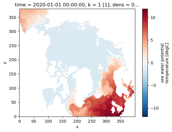
What’s next#
Lazy loading & chunking — open multi-year archives without loading data into memory, choose chunk sizes, and filter to only the variables you need.
Working with HYCOM data — slicing, plotting, time operations,
groupby, and seasonal analysis once the Dataset is open.