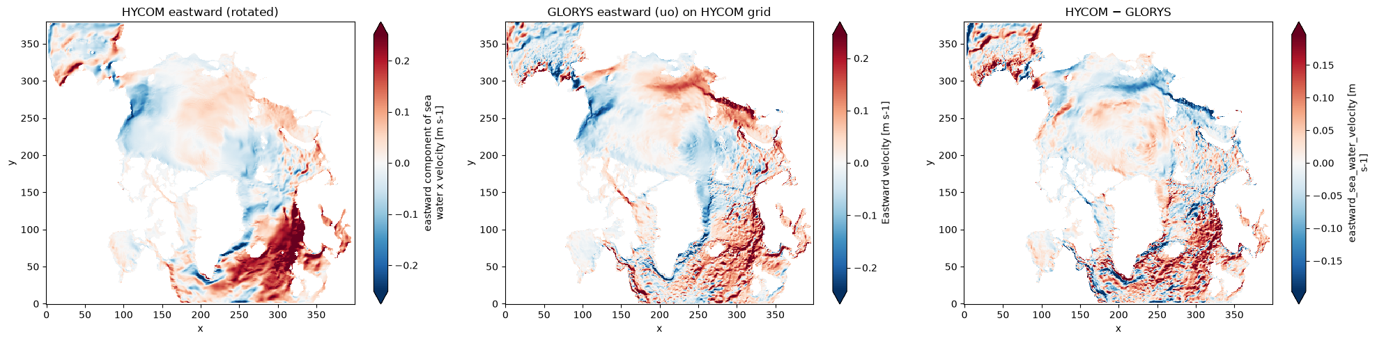
Regridding#
HYCOM output lives on two non-standard grids:
Horizontal — curvilinear, with 2-D
lon/latand velocities on a staggered, rotated C-grid.Vertical — hybrid isopycnal, with layer thicknesses stored as pressure (
thknss).
xhycom.regrid maps both onto a regular lon/lat/depth grid — conservatively by default (area-conservative horizontally, depth-integral-conserving vertically) — for comparison with reanalyses like GLORYS.
Install#
pip install xhycom # vertical regridding (xgcm + Dask) is included
Horizontal regridding also needs xESMF (conda-only ESMF backend, kept optional since it can conflict with other ESMF installs). Create the conda environment first, then install xhycom into it — don’t pip install xhycom into a plain env and expect xESMF to appear:
conda env create -f ci/environment-regrid.yml
import numpy as np
import xarray as xr
import xhycom
import matplotlib.pyplot as plt
grid = "/cluster/home/nlo043/NERSC-HYCOM-CICE/TP2a0.10/topo/regional.grid"
DATA_PATH = "/nird/datalake/NS9481K/shuang/TP2_output/expt_02.8/"
Open HYCOM output#
Load the 2020 archive year with its grid. postprocess=True converts thicknesses and SSH to metres, and chunks={"time": 1} loads the data lazily, one time step at a time. Learn more about choosing chunk sizes and working with lazy-loaded data in Lazy loading & chunking.
ds = xhycom.open_mfdataset(DATA_PATH + "archm.2020*", grid=grid, chunks={"time": 1}, postprocess=True)
ds
<xarray.Dataset> Size: 1TB
Dimensions:     (y: 380, x: 400, time: 366, k: 50, ki: 51)
Coordinates:
    lon         (y, x) float64 1MB dask.array<chunksize=(380, 400), meta=np.ndarray>
    lat         (y, x) float64 1MB dask.array<chunksize=(380, 400), meta=np.ndarray>
    lon_u       (y, x) float64 1MB dask.array<chunksize=(380, 400), meta=np.ndarray>
    lat_u       (y, x) float64 1MB dask.array<chunksize=(380, 400), meta=np.ndarray>
    lon_v       (y, x) float64 1MB dask.array<chunksize=(380, 400), meta=np.ndarray>
    lat_v       (y, x) float64 1MB dask.array<chunksize=(380, 400), meta=np.ndarray>
  * time        (time) object 3kB 2020-01-01 00:00:00 ... 2020-12-31 00:00:00
  * k           (k) int64 400B 1 2 3 4 5 6 7 8 9 ... 42 43 44 45 46 47 48 49 50
    dens        (k) float64 400B dask.array<chunksize=(50,), meta=np.ndarray>
  * ki          (ki) int64 408B 0 1 2 3 4 5 6 7 8 ... 42 43 44 45 46 47 48 49 50
Dimensions without coordinates: y, x
Data variables: (12/83)
    montg1      (time, y, x) float64 445MB dask.array<chunksize=(1, 380, 400), meta=np.ndarray>
    srfhgt      (time, y, x) float64 445MB dask.array<chunksize=(1, 380, 400), meta=np.ndarray>
    oneta       (time, y, x) float64 445MB dask.array<chunksize=(1, 380, 400), meta=np.ndarray>
    surflx      (time, y, x) float64 445MB dask.array<chunksize=(1, 380, 400), meta=np.ndarray>
    wtrflx      (time, y, x) float64 445MB dask.array<chunksize=(1, 380, 400), meta=np.ndarray>
    salflx      (time, y, x) float64 445MB dask.array<chunksize=(1, 380, 400), meta=np.ndarray>
    ...          ...
    CO2_wind    (time, y, x) float64 445MB dask.array<chunksize=(1, 380, 400), meta=np.ndarray>
    ECO_bots    (time, y, x) float64 445MB dask.array<chunksize=(1, 380, 400), meta=np.ndarray>
    surface__1  (time, y, x) float64 445MB dask.array<chunksize=(1, 380, 400), meta=np.ndarray>
    surface__2  (time, y, x) float64 445MB dask.array<chunksize=(1, 380, 400), meta=np.ndarray>
    si_u        (time, y, x) float64 445MB dask.array<chunksize=(1, 380, 400), meta=np.ndarray>
    si_v        (time, y, x) float64 445MB dask.array<chunksize=(1, 380, 400), meta=np.ndarray>
Attributes:
    iversn:        23
    iexpt:         28
    yrflag:        3
archive_type: mean- y: 380
- x: 400
- time: 366
- k: 50
- ki: 51
- lon(y, x)float64dask.array<chunksize=(380, 400), meta=np.ndarray>
- long_name :
- longitude (T-point)
- units :
- degrees_east
- standard_name :
- longitude
Array Chunk Bytes 1.16 MiB 1.16 MiB Shape (380, 400) (380, 400) Dask graph 1 chunks in 1 graph layer Data type float64 numpy.ndarray - lat(y, x)float64dask.array<chunksize=(380, 400), meta=np.ndarray>
- long_name :
- latitude (T-point)
- units :
- degrees_north
- standard_name :
- latitude
Array Chunk Bytes 1.16 MiB 1.16 MiB Shape (380, 400) (380, 400) Dask graph 1 chunks in 1 graph layer Data type float64 numpy.ndarray - lon_u(y, x)float64dask.array<chunksize=(380, 400), meta=np.ndarray>
- long_name :
- longitude (U-point)
- units :
- degrees_east
Array Chunk Bytes 1.16 MiB 1.16 MiB Shape (380, 400) (380, 400) Dask graph 1 chunks in 1 graph layer Data type float64 numpy.ndarray - lat_u(y, x)float64dask.array<chunksize=(380, 400), meta=np.ndarray>
- long_name :
- latitude (U-point)
- units :
- degrees_north
Array Chunk Bytes 1.16 MiB 1.16 MiB Shape (380, 400) (380, 400) Dask graph 1 chunks in 1 graph layer Data type float64 numpy.ndarray - lon_v(y, x)float64dask.array<chunksize=(380, 400), meta=np.ndarray>
- long_name :
- longitude (V-point)
- units :
- degrees_east
Array Chunk Bytes 1.16 MiB 1.16 MiB Shape (380, 400) (380, 400) Dask graph 1 chunks in 1 graph layer Data type float64 numpy.ndarray - lat_v(y, x)float64dask.array<chunksize=(380, 400), meta=np.ndarray>
- long_name :
- latitude (V-point)
- units :
- degrees_north
Array Chunk Bytes 1.16 MiB 1.16 MiB Shape (380, 400) (380, 400) Dask graph 1 chunks in 1 graph layer Data type float64 numpy.ndarray - time(time)object2020-01-01 00:00:00 ... 2020-12-...
- long_name :
- time
- axis :
- T
array([cftime.DatetimeGregorian(2020, 1, 1, 0, 0, 0, 0, has_year_zero=False), cftime.DatetimeGregorian(2020, 1, 2, 0, 0, 0, 0, has_year_zero=False), cftime.DatetimeGregorian(2020, 1, 3, 0, 0, 0, 0, has_year_zero=False), ..., cftime.DatetimeGregorian(2020, 12, 29, 0, 0, 0, 0, has_year_zero=False), cftime.DatetimeGregorian(2020, 12, 30, 0, 0, 0, 0, has_year_zero=False), cftime.DatetimeGregorian(2020, 12, 31, 0, 0, 0, 0, has_year_zero=False)], shape=(366,), dtype=object) - k(k)int641 2 3 4 5 6 7 ... 45 46 47 48 49 50
- long_name :
- layer index
- units :
- 1
- axis :
- Z
array([ 1, 2, 3, 4, 5, 6, 7, 8, 9, 10, 11, 12, 13, 14, 15, 16, 17, 18, 19, 20, 21, 22, 23, 24, 25, 26, 27, 28, 29, 30, 31, 32, 33, 34, 35, 36, 37, 38, 39, 40, 41, 42, 43, 44, 45, 46, 47, 48, 49, 50]) - dens(k)float64dask.array<chunksize=(50,), meta=np.ndarray>
- long_name :
- target sigma-2 layer density
- units :
- kg m-3
Array Chunk Bytes 400 B 400 B Shape (50,) (50,) Dask graph 1 chunks in 1 graph layer Data type float64 numpy.ndarray - ki(ki)int640 1 2 3 4 5 6 ... 45 46 47 48 49 50
- long_name :
- layer interface index
- units :
- 1
- axis :
- Z
array([ 0,  1,  2,  3,  4,  5,  6,  7,  8,  9, 10, 11, 12, 13, 14, 15, 16, 17,
       18, 19, 20, 21, 22, 23, 24, 25, 26, 27, 28, 29, 30, 31, 32, 33, 34, 35,
       36, 37, 38, 39, 40, 41, 42, 43, 44, 45, 46, 47, 48, 49, 50])
- montg1(time, y, x)float64dask.array<chunksize=(1, 380, 400), meta=np.ndarray>
- long_name :
- Montgomery potential
- units :
- m2 s-2
Array Chunk Bytes 424.44 MiB 1.16 MiB Shape (366, 380, 400) (1, 380, 400) Dask graph 366 chunks in 733 graph layers Data type float64 numpy.ndarray - srfhgt(time, y, x)float64dask.array<chunksize=(1, 380, 400), meta=np.ndarray>
- long_name :
- sea surface height
- units :
- m
- comment :
- converted from Pa (factor 0.101978)
Array Chunk Bytes 424.44 MiB 1.16 MiB Shape (366, 380, 400) (1, 380, 400) Dask graph 366 chunks in 734 graph layers Data type float64 numpy.ndarray - oneta(time, y, x)float64dask.array<chunksize=(1, 380, 400), meta=np.ndarray>
- long_name :
- free surface elevation
- units :
- m
Array Chunk Bytes 424.44 MiB 1.16 MiB Shape (366, 380, 400) (1, 380, 400) Dask graph 366 chunks in 733 graph layers Data type float64 numpy.ndarray - surflx(time, y, x)float64dask.array<chunksize=(1, 380, 400), meta=np.ndarray>
- long_name :
- net surface heat flux
- units :
- W m-2
Array Chunk Bytes 424.44 MiB 1.16 MiB Shape (366, 380, 400) (1, 380, 400) Dask graph 366 chunks in 733 graph layers Data type float64 numpy.ndarray - wtrflx(time, y, x)float64dask.array<chunksize=(1, 380, 400), meta=np.ndarray>
- long_name :
- net surface freshwater flux
- units :
- m s-1
Array Chunk Bytes 424.44 MiB 1.16 MiB Shape (366, 380, 400) (1, 380, 400) Dask graph 366 chunks in 733 graph layers Data type float64 numpy.ndarray - salflx(time, y, x)float64dask.array<chunksize=(1, 380, 400), meta=np.ndarray>
- long_name :
- surface salt flux
- units :
- PSU m s-1
Array Chunk Bytes 424.44 MiB 1.16 MiB Shape (366, 380, 400) (1, 380, 400) Dask graph 366 chunks in 733 graph layers Data type float64 numpy.ndarray - bl_dpth(time, y, x)float64dask.array<chunksize=(1, 380, 400), meta=np.ndarray>
- long_name :
- boundary layer depth
- units :
- m
- comment :
- converted from Pa (factor 0.000101978)
Array Chunk Bytes 424.44 MiB 1.16 MiB Shape (366, 380, 400) (1, 380, 400) Dask graph 366 chunks in 734 graph layers Data type float64 numpy.ndarray - mix_dpth(time, y, x)float64dask.array<chunksize=(1, 380, 400), meta=np.ndarray>
- long_name :
- mixed layer depth
- units :
- m
- comment :
- converted from Pa (factor 0.000101978)
Array Chunk Bytes 424.44 MiB 1.16 MiB Shape (366, 380, 400) (1, 380, 400) Dask graph 366 chunks in 734 graph layers Data type float64 numpy.ndarray - tmix(time, y, x)float64dask.array<chunksize=(1, 380, 400), meta=np.ndarray>
- long_name :
- mixed layer temperature
- units :
- degC
Array Chunk Bytes 424.44 MiB 1.16 MiB Shape (366, 380, 400) (1, 380, 400) Dask graph 366 chunks in 733 graph layers Data type float64 numpy.ndarray - smix(time, y, x)float64dask.array<chunksize=(1, 380, 400), meta=np.ndarray>
- long_name :
- mixed layer salinity
- units :
- PSU
Array Chunk Bytes 424.44 MiB 1.16 MiB Shape (366, 380, 400) (1, 380, 400) Dask graph 366 chunks in 733 graph layers Data type float64 numpy.ndarray - thmix(time, y, x)float64dask.array<chunksize=(1, 380, 400), meta=np.ndarray>
- long_name :
- mixed layer thickness
- units :
- m
- comment :
- converted from Pa (factor 0.000101978)
Array Chunk Bytes 424.44 MiB 1.16 MiB Shape (366, 380, 400) (1, 380, 400) Dask graph 366 chunks in 734 graph layers Data type float64 numpy.ndarray - umix(time, y, x)float64dask.array<chunksize=(1, 380, 400), meta=np.ndarray>
- long_name :
- mixed layer x velocity
- units :
- m s-1
Array Chunk Bytes 424.44 MiB 1.16 MiB Shape (366, 380, 400) (1, 380, 400) Dask graph 366 chunks in 733 graph layers Data type float64 numpy.ndarray - vmix(time, y, x)float64dask.array<chunksize=(1, 380, 400), meta=np.ndarray>
- long_name :
- mixed layer y velocity
- units :
- m s-1
Array Chunk Bytes 424.44 MiB 1.16 MiB Shape (366, 380, 400) (1, 380, 400) Dask graph 366 chunks in 733 graph layers Data type float64 numpy.ndarray - kemix(time, y, x)float64dask.array<chunksize=(1, 380, 400), meta=np.ndarray>
- long_name :
- mixed layer kinetic energy
- units :
- m2 s-2
Array Chunk Bytes 424.44 MiB 1.16 MiB Shape (366, 380, 400) (1, 380, 400) Dask graph 366 chunks in 733 graph layers Data type float64 numpy.ndarray - covice(time, y, x)float64dask.array<chunksize=(1, 380, 400), meta=np.ndarray>
- long_name :
- sea ice coverage fraction
- units :
- 1
Array Chunk Bytes 424.44 MiB 1.16 MiB Shape (366, 380, 400) (1, 380, 400) Dask graph 366 chunks in 733 graph layers Data type float64 numpy.ndarray - thkice(time, y, x)float64dask.array<chunksize=(1, 380, 400), meta=np.ndarray>
- long_name :
- sea ice thickness
- units :
- m
Array Chunk Bytes 424.44 MiB 1.16 MiB Shape (366, 380, 400) (1, 380, 400) Dask graph 366 chunks in 733 graph layers Data type float64 numpy.ndarray - temice(time, y, x)float64dask.array<chunksize=(1, 380, 400), meta=np.ndarray>
- long_name :
- sea ice surface temperature
- units :
- degC
Array Chunk Bytes 424.44 MiB 1.16 MiB Shape (366, 380, 400) (1, 380, 400) Dask graph 366 chunks in 733 graph layers Data type float64 numpy.ndarray - u_btrop(time, y, x)float64dask.array<chunksize=(1, 380, 400), meta=np.ndarray>
- long_name :
- barotropic x velocity
- units :
- m s-1
Array Chunk Bytes 424.44 MiB 1.16 MiB Shape (366, 380, 400) (1, 380, 400) Dask graph 366 chunks in 733 graph layers Data type float64 numpy.ndarray - v_btrop(time, y, x)float64dask.array<chunksize=(1, 380, 400), meta=np.ndarray>
- long_name :
- barotropic y velocity
- units :
- m s-1
Array Chunk Bytes 424.44 MiB 1.16 MiB Shape (366, 380, 400) (1, 380, 400) Dask graph 366 chunks in 733 graph layers Data type float64 numpy.ndarray - kebtrop(time, y, x)float64dask.array<chunksize=(1, 380, 400), meta=np.ndarray>
- long_name :
- barotropic kinetic energy
- units :
- m2 s-2
Array Chunk Bytes 424.44 MiB 1.16 MiB Shape (366, 380, 400) (1, 380, 400) Dask graph 366 chunks in 733 graph layers Data type float64 numpy.ndarray - u-vel.(time, k, y, x)float64dask.array<chunksize=(1, 50, 380, 400), meta=np.ndarray>
- long_name :
- sea water x velocity
- units :
- m s-1
- hycom_velocity :
- total
- comment :
- total current (baroclinic + barotropic); the barotropic part was summed in when the archm time mean was formed
Array Chunk Bytes 20.72 GiB 57.98 MiB Shape (366, 50, 380, 400) (1, 50, 380, 400) Dask graph 366 chunks in 733 graph layers Data type float64 numpy.ndarray - v-vel.(time, k, y, x)float64dask.array<chunksize=(1, 50, 380, 400), meta=np.ndarray>
- long_name :
- sea water y velocity
- units :
- m s-1
- hycom_velocity :
- total
- comment :
- total current (baroclinic + barotropic); the barotropic part was summed in when the archm time mean was formed
Array Chunk Bytes 20.72 GiB 57.98 MiB Shape (366, 50, 380, 400) (1, 50, 380, 400) Dask graph 366 chunks in 733 graph layers Data type float64 numpy.ndarray - k.e.(time, k, y, x)float64dask.array<chunksize=(1, 50, 380, 400), meta=np.ndarray>
- long_name :
- kinetic energy
- units :
- m2 s-2
Array Chunk Bytes 20.72 GiB 57.98 MiB Shape (366, 50, 380, 400) (1, 50, 380, 400) Dask graph 366 chunks in 733 graph layers Data type float64 numpy.ndarray - thknss(time, k, y, x)float64dask.array<chunksize=(1, 50, 380, 400), meta=np.ndarray>
- long_name :
- layer thickness
- units :
- m
- comment :
- converted from Pa (factor 0.000101978)
Array Chunk Bytes 20.72 GiB 57.98 MiB Shape (366, 50, 380, 400) (1, 50, 380, 400) Dask graph 366 chunks in 734 graph layers Data type float64 numpy.ndarray - temp(time, k, y, x)float64dask.array<chunksize=(1, 50, 380, 400), meta=np.ndarray>
- long_name :
- sea water potential temperature
- units :
- degC
Array Chunk Bytes 20.72 GiB 57.98 MiB Shape (366, 50, 380, 400) (1, 50, 380, 400) Dask graph 366 chunks in 733 graph layers Data type float64 numpy.ndarray - salin(time, k, y, x)float64dask.array<chunksize=(1, 50, 380, 400), meta=np.ndarray>
- long_name :
- sea water salinity
- units :
- PSU
Array Chunk Bytes 20.72 GiB 57.98 MiB Shape (366, 50, 380, 400) (1, 50, 380, 400) Dask graph 366 chunks in 733 graph layers Data type float64 numpy.ndarray - density(time, k, y, x)float64dask.array<chunksize=(1, 50, 380, 400), meta=np.ndarray>
- long_name :
- sea water potential density (sigma-2)
- units :
- kg m-3
Array Chunk Bytes 20.72 GiB 57.98 MiB Shape (366, 50, 380, 400) (1, 50, 380, 400) Dask graph 366 chunks in 733 graph layers Data type float64 numpy.ndarray - CO2_c(time, k, y, x)float64dask.array<chunksize=(1, 50, 380, 400), meta=np.ndarray>
- long_name :
- dissolved inorganic carbon
- units :
- mmol C m-3
Array Chunk Bytes 20.72 GiB 57.98 MiB Shape (366, 50, 380, 400) (1, 50, 380, 400) Dask graph 366 chunks in 733 graph layers Data type float64 numpy.ndarray - CO2_TA(time, k, y, x)float64dask.array<chunksize=(1, 50, 380, 400), meta=np.ndarray>
- long_name :
- total alkalinity
- units :
- mmol eq m-3
Array Chunk Bytes 20.72 GiB 57.98 MiB Shape (366, 50, 380, 400) (1, 50, 380, 400) Dask graph 366 chunks in 733 graph layers Data type float64 numpy.ndarray - ECO_no3(time, k, y, x)float64dask.array<chunksize=(1, 50, 380, 400), meta=np.ndarray>
- long_name :
- nitrate
- units :
- mmol N m-3
Array Chunk Bytes 20.72 GiB 57.98 MiB Shape (366, 50, 380, 400) (1, 50, 380, 400) Dask graph 366 chunks in 733 graph layers Data type float64 numpy.ndarray - ECO_nh4(time, k, y, x)float64dask.array<chunksize=(1, 50, 380, 400), meta=np.ndarray>
- long_name :
- ammonium
- units :
- mmol N m-3
Array Chunk Bytes 20.72 GiB 57.98 MiB Shape (366, 50, 380, 400) (1, 50, 380, 400) Dask graph 366 chunks in 733 graph layers Data type float64 numpy.ndarray - ECO_pho(time, k, y, x)float64dask.array<chunksize=(1, 50, 380, 400), meta=np.ndarray>
- long_name :
- phosphate
- units :
- mmol P m-3
Array Chunk Bytes 20.72 GiB 57.98 MiB Shape (366, 50, 380, 400) (1, 50, 380, 400) Dask graph 366 chunks in 733 graph layers Data type float64 numpy.ndarray - ECO_sil(time, k, y, x)float64dask.array<chunksize=(1, 50, 380, 400), meta=np.ndarray>
- long_name :
- silicate
- units :
- mmol Si m-3
Array Chunk Bytes 20.72 GiB 57.98 MiB Shape (366, 50, 380, 400) (1, 50, 380, 400) Dask graph 366 chunks in 733 graph layers Data type float64 numpy.ndarray - ECO_oxy(time, k, y, x)float64dask.array<chunksize=(1, 50, 380, 400), meta=np.ndarray>
- long_name :
- dissolved oxygen
- units :
- mmol O m-3
Array Chunk Bytes 20.72 GiB 57.98 MiB Shape (366, 50, 380, 400) (1, 50, 380, 400) Dask graph 366 chunks in 733 graph layers Data type float64 numpy.ndarray - ECO_fla(time, k, y, x)float64dask.array<chunksize=(1, 50, 380, 400), meta=np.ndarray>
- long_name :
- flagellate carbon
- units :
- mmol C m-3
Array Chunk Bytes 20.72 GiB 57.98 MiB Shape (366, 50, 380, 400) (1, 50, 380, 400) Dask graph 366 chunks in 733 graph layers Data type float64 numpy.ndarray - ECO_dia(time, k, y, x)float64dask.array<chunksize=(1, 50, 380, 400), meta=np.ndarray>
- long_name :
- diatom carbon
- units :
- mmol C m-3
Array Chunk Bytes 20.72 GiB 57.98 MiB Shape (366, 50, 380, 400) (1, 50, 380, 400) Dask graph 366 chunks in 733 graph layers Data type float64 numpy.ndarray - ECO_ccl(time, k, y, x)float64dask.array<chunksize=(1, 50, 380, 400), meta=np.ndarray>
- long_name :
- coccolithophore carbon
- units :
- mmol C m-3
Array Chunk Bytes 20.72 GiB 57.98 MiB Shape (366, 50, 380, 400) (1, 50, 380, 400) Dask graph 366 chunks in 733 graph layers Data type float64 numpy.ndarray - ECO_cclc(time, k, y, x)float64dask.array<chunksize=(1, 50, 380, 400), meta=np.ndarray>
- long_name :
- coccolithophore calcite carbon
- units :
- mmol C m-3
Array Chunk Bytes 20.72 GiB 57.98 MiB Shape (366, 50, 380, 400) (1, 50, 380, 400) Dask graph 366 chunks in 733 graph layers Data type float64 numpy.ndarray - ECO_caco(time, k, y, x)float64dask.array<chunksize=(1, 50, 380, 400), meta=np.ndarray>
- long_name :
- particulate inorganic carbon (calcite)
- units :
- mmol C m-3
Array Chunk Bytes 20.72 GiB 57.98 MiB Shape (366, 50, 380, 400) (1, 50, 380, 400) Dask graph 366 chunks in 733 graph layers Data type float64 numpy.ndarray - ECO_diac(time, k, y, x)float64dask.array<chunksize=(1, 50, 380, 400), meta=np.ndarray>
- long_name :
- diatom calcite carbon
- units :
- mmol C m-3
Array Chunk Bytes 20.72 GiB 57.98 MiB Shape (366, 50, 380, 400) (1, 50, 380, 400) Dask graph 366 chunks in 733 graph layers Data type float64 numpy.ndarray - ECO_flac(time, k, y, x)float64dask.array<chunksize=(1, 50, 380, 400), meta=np.ndarray>
- long_name :
- flagellate calcite carbon
- units :
- mmol C m-3
Array Chunk Bytes 20.72 GiB 57.98 MiB Shape (366, 50, 380, 400) (1, 50, 380, 400) Dask graph 366 chunks in 733 graph layers Data type float64 numpy.ndarray - ECO_micr(time, k, y, x)float64dask.array<chunksize=(1, 50, 380, 400), meta=np.ndarray>
- long_name :
- microzooplankton carbon
- units :
- mmol C m-3
Array Chunk Bytes 20.72 GiB 57.98 MiB Shape (366, 50, 380, 400) (1, 50, 380, 400) Dask graph 366 chunks in 733 graph layers Data type float64 numpy.ndarray - ECO_meso(time, k, y, x)float64dask.array<chunksize=(1, 50, 380, 400), meta=np.ndarray>
- long_name :
- mesozooplankton carbon
- units :
- mmol C m-3
Array Chunk Bytes 20.72 GiB 57.98 MiB Shape (366, 50, 380, 400) (1, 50, 380, 400) Dask graph 366 chunks in 733 graph layers Data type float64 numpy.ndarray - ECO_det(time, k, y, x)float64dask.array<chunksize=(1, 50, 380, 400), meta=np.ndarray>
- long_name :
- detritus carbon
- units :
- mmol C m-3
Array Chunk Bytes 20.72 GiB 57.98 MiB Shape (366, 50, 380, 400) (1, 50, 380, 400) Dask graph 366 chunks in 733 graph layers Data type float64 numpy.ndarray - ECO_opa(time, k, y, x)float64dask.array<chunksize=(1, 50, 380, 400), meta=np.ndarray>
- long_name :
- opal (biogenic silica)
- units :
- mmol Si m-3
Array Chunk Bytes 20.72 GiB 57.98 MiB Shape (366, 50, 380, 400) (1, 50, 380, 400) Dask graph 366 chunks in 733 graph layers Data type float64 numpy.ndarray - ECO_dom(time, k, y, x)float64dask.array<chunksize=(1, 50, 380, 400), meta=np.ndarray>
- long_name :
- dissolved organic matter carbon
- units :
- mmol C m-3
Array Chunk Bytes 20.72 GiB 57.98 MiB Shape (366, 50, 380, 400) (1, 50, 380, 400) Dask graph 366 chunks in 733 graph layers Data type float64 numpy.ndarray - ECO_dsnk(time, k, y, x)float64dask.array<chunksize=(1, 50, 380, 400), meta=np.ndarray>
- long_name :
- detritus sinking flux
- units :
- mmol C m-2 s-1
Array Chunk Bytes 20.72 GiB 57.98 MiB Shape (366, 50, 380, 400) (1, 50, 380, 400) Dask graph 366 chunks in 733 graph layers Data type float64 numpy.ndarray - CO2_pH(time, k, y, x)float64dask.array<chunksize=(1, 50, 380, 400), meta=np.ndarray>
- long_name :
- seawater pH
- units :
- 1
Array Chunk Bytes 20.72 GiB 57.98 MiB Shape (366, 50, 380, 400) (1, 50, 380, 400) Dask graph 366 chunks in 733 graph layers Data type float64 numpy.ndarray - CO2_pCO2(time, k, y, x)float64dask.array<chunksize=(1, 50, 380, 400), meta=np.ndarray>
- long_name :
- partial pressure of CO2
- units :
- uatm
Array Chunk Bytes 20.72 GiB 57.98 MiB Shape (366, 50, 380, 400) (1, 50, 380, 400) Dask graph 366 chunks in 733 graph layers Data type float64 numpy.ndarray - CO2_Carb_1(time, k, y, x)float64dask.array<chunksize=(1, 50, 380, 400), meta=np.ndarray>
- long_name :
- carbonate concentration
- units :
- mmol C m-3
Array Chunk Bytes 20.72 GiB 57.98 MiB Shape (366, 50, 380, 400) (1, 50, 380, 400) Dask graph 366 chunks in 733 graph layers Data type float64 numpy.ndarray - CO2_BiCa(time, k, y, x)float64dask.array<chunksize=(1, 50, 380, 400), meta=np.ndarray>
- long_name :
- bicarbonate concentration
- units :
- mmol C m-3
Array Chunk Bytes 20.72 GiB 57.98 MiB Shape (366, 50, 380, 400) (1, 50, 380, 400) Dask graph 366 chunks in 733 graph layers Data type float64 numpy.ndarray - CO2_Carb_2(time, k, y, x)float64dask.array<chunksize=(1, 50, 380, 400), meta=np.ndarray>
- long_name :
- carbonate concentration
- units :
- mmol C m-3
Array Chunk Bytes 20.72 GiB 57.98 MiB Shape (366, 50, 380, 400) (1, 50, 380, 400) Dask graph 366 chunks in 733 graph layers Data type float64 numpy.ndarray - CO2_Om_c(time, k, y, x)float64dask.array<chunksize=(1, 50, 380, 400), meta=np.ndarray>
- long_name :
- calcite saturation state (Omega)
- units :
- 1
Array Chunk Bytes 20.72 GiB 57.98 MiB Shape (366, 50, 380, 400) (1, 50, 380, 400) Dask graph 366 chunks in 733 graph layers Data type float64 numpy.ndarray - CO2_Om_a(time, k, y, x)float64dask.array<chunksize=(1, 50, 380, 400), meta=np.ndarray>
- long_name :
- aragonite saturation state (Omega)
- units :
- 1
Array Chunk Bytes 20.72 GiB 57.98 MiB Shape (366, 50, 380, 400) (1, 50, 380, 400) Dask graph 366 chunks in 733 graph layers Data type float64 numpy.ndarray - ECO_prim(time, k, y, x)float64dask.array<chunksize=(1, 50, 380, 400), meta=np.ndarray>
- long_name :
- primary production
- units :
- mmol C m-3 s-1
Array Chunk Bytes 20.72 GiB 57.98 MiB Shape (366, 50, 380, 400) (1, 50, 380, 400) Dask graph 366 chunks in 733 graph layers Data type float64 numpy.ndarray - ECO_secp(time, k, y, x)float64dask.array<chunksize=(1, 50, 380, 400), meta=np.ndarray>
- long_name :
- secondary production
- units :
- mmol C m-3 s-1
Array Chunk Bytes 20.72 GiB 57.98 MiB Shape (366, 50, 380, 400) (1, 50, 380, 400) Dask graph 366 chunks in 733 graph layers Data type float64 numpy.ndarray - ECO_netp(time, k, y, x)float64dask.array<chunksize=(1, 50, 380, 400), meta=np.ndarray>
- long_name :
- net primary production
- units :
- mmol C m-3 s-1
Array Chunk Bytes 20.72 GiB 57.98 MiB Shape (366, 50, 380, 400) (1, 50, 380, 400) Dask graph 366 chunks in 733 graph layers Data type float64 numpy.ndarray - ECO_parm(time, k, y, x)float64dask.array<chunksize=(1, 50, 380, 400), meta=np.ndarray>
- long_name :
- BGC parameter field
- units :
- 1
Array Chunk Bytes 20.72 GiB 57.98 MiB Shape (366, 50, 380, 400) (1, 50, 380, 400) Dask graph 366 chunks in 733 graph layers Data type float64 numpy.ndarray - ECO_Nlim(time, k, y, x)float64dask.array<chunksize=(1, 50, 380, 400), meta=np.ndarray>
- long_name :
- nitrogen limitation factor
- units :
- 1
Array Chunk Bytes 20.72 GiB 57.98 MiB Shape (366, 50, 380, 400) (1, 50, 380, 400) Dask graph 366 chunks in 733 graph layers Data type float64 numpy.ndarray - ECO_Plim(time, k, y, x)float64dask.array<chunksize=(1, 50, 380, 400), meta=np.ndarray>
- long_name :
- phosphorus limitation factor
- units :
- 1
Array Chunk Bytes 20.72 GiB 57.98 MiB Shape (366, 50, 380, 400) (1, 50, 380, 400) Dask graph 366 chunks in 733 graph layers Data type float64 numpy.ndarray - ECO_Slim(time, k, y, x)float64dask.array<chunksize=(1, 50, 380, 400), meta=np.ndarray>
- long_name :
- silicate limitation factor
- units :
- 1
Array Chunk Bytes 20.72 GiB 57.98 MiB Shape (366, 50, 380, 400) (1, 50, 380, 400) Dask graph 366 chunks in 733 graph layers Data type float64 numpy.ndarray - ECO_Llim(time, k, y, x)float64dask.array<chunksize=(1, 50, 380, 400), meta=np.ndarray>
- long_name :
- light limitation factor
- units :
- 1
Array Chunk Bytes 20.72 GiB 57.98 MiB Shape (366, 50, 380, 400) (1, 50, 380, 400) Dask graph 366 chunks in 733 graph layers Data type float64 numpy.ndarray - ECO_deni(time, k, y, x)float64dask.array<chunksize=(1, 50, 380, 400), meta=np.ndarray>
- long_name :
- denitrification
- units :
- mmol N m-3 s-1
Array Chunk Bytes 20.72 GiB 57.98 MiB Shape (366, 50, 380, 400) (1, 50, 380, 400) Dask graph 366 chunks in 733 graph layers Data type float64 numpy.ndarray - ECO_snks(time, k, y, x)float64dask.array<chunksize=(1, 50, 380, 400), meta=np.ndarray>
- long_name :
- sinking rate
- units :
- m d-1
Array Chunk Bytes 20.72 GiB 57.98 MiB Shape (366, 50, 380, 400) (1, 50, 380, 400) Dask graph 366 chunks in 733 graph layers Data type float64 numpy.ndarray - ECO_c2ch_1(time, k, y, x)float64dask.array<chunksize=(1, 50, 380, 400), meta=np.ndarray>
- long_name :
- carbon to chlorophyll ratio
- units :
- g C g-1 Chl
Array Chunk Bytes 20.72 GiB 57.98 MiB Shape (366, 50, 380, 400) (1, 50, 380, 400) Dask graph 366 chunks in 733 graph layers Data type float64 numpy.ndarray - ECO_c2ch_2(time, k, y, x)float64dask.array<chunksize=(1, 50, 380, 400), meta=np.ndarray>
- long_name :
- carbon to chlorophyll ratio
- units :
- g C g-1 Chl
Array Chunk Bytes 20.72 GiB 57.98 MiB Shape (366, 50, 380, 400) (1, 50, 380, 400) Dask graph 366 chunks in 733 graph layers Data type float64 numpy.ndarray - ECO_c2ch_3(time, k, y, x)float64dask.array<chunksize=(1, 50, 380, 400), meta=np.ndarray>
- long_name :
- carbon to chlorophyll ratio
- units :
- g C g-1 Chl
Array Chunk Bytes 20.72 GiB 57.98 MiB Shape (366, 50, 380, 400) (1, 50, 380, 400) Dask graph 366 chunks in 733 graph layers Data type float64 numpy.ndarray - light_sw(time, k, y, x)float64dask.array<chunksize=(1, 50, 380, 400), meta=np.ndarray>
- long_name :
- shortwave irradiance in water
- units :
- W m-2
Array Chunk Bytes 20.72 GiB 57.98 MiB Shape (366, 50, 380, 400) (1, 50, 380, 400) Dask graph 366 chunks in 733 graph layers Data type float64 numpy.ndarray - light_pa(time, ki, y, x)float64dask.array<chunksize=(1, 51, 380, 400), meta=np.ndarray>
- long_name :
- PAR irradiance
- units :
- W m-2
Array Chunk Bytes 21.14 GiB 59.14 MiB Shape (366, 51, 380, 400) (1, 51, 380, 400) Dask graph 366 chunks in 733 graph layers Data type float64 numpy.ndarray - attenuat(time, k, y, x)float64dask.array<chunksize=(1, 50, 380, 400), meta=np.ndarray>
- long_name :
- light attenuation coefficient
- units :
- m-1
Array Chunk Bytes 20.72 GiB 57.98 MiB Shape (366, 50, 380, 400) (1, 50, 380, 400) Dask graph 366 chunks in 733 graph layers Data type float64 numpy.ndarray - total_ch(time, k, y, x)float64dask.array<chunksize=(1, 50, 380, 400), meta=np.ndarray>
- long_name :
- total chlorophyll
- units :
- mg Chl m-3
Array Chunk Bytes 20.72 GiB 57.98 MiB Shape (366, 50, 380, 400) (1, 50, 380, 400) Dask graph 366 chunks in 733 graph layers Data type float64 numpy.ndarray - total_ca(time, k, y, x)float64dask.array<chunksize=(1, 50, 380, 400), meta=np.ndarray>
- long_name :
- total carbon
- units :
- mmol C m-3
Array Chunk Bytes 20.72 GiB 57.98 MiB Shape (366, 50, 380, 400) (1, 50, 380, 400) Dask graph 366 chunks in 733 graph layers Data type float64 numpy.ndarray - ECO_sed4(time, y, x)float64dask.array<chunksize=(1, 380, 400), meta=np.ndarray>
- long_name :
- sediment pool 4
- units :
- mmol m-2
Array Chunk Bytes 424.44 MiB 1.16 MiB Shape (366, 380, 400) (1, 380, 400) Dask graph 366 chunks in 733 graph layers Data type float64 numpy.ndarray - ECO_sed1(time, y, x)float64dask.array<chunksize=(1, 380, 400), meta=np.ndarray>
- long_name :
- sediment pool 1
- units :
- mmol m-2
Array Chunk Bytes 424.44 MiB 1.16 MiB Shape (366, 380, 400) (1, 380, 400) Dask graph 366 chunks in 733 graph layers Data type float64 numpy.ndarray - ECO_sed2(time, y, x)float64dask.array<chunksize=(1, 380, 400), meta=np.ndarray>
- long_name :
- sediment pool 2
- units :
- mmol m-2
Array Chunk Bytes 424.44 MiB 1.16 MiB Shape (366, 380, 400) (1, 380, 400) Dask graph 366 chunks in 733 graph layers Data type float64 numpy.ndarray - ECO_sed3(time, y, x)float64dask.array<chunksize=(1, 380, 400), meta=np.ndarray>
- long_name :
- sediment pool 3
- units :
- mmol m-2
Array Chunk Bytes 424.44 MiB 1.16 MiB Shape (366, 380, 400) (1, 380, 400) Dask graph 366 chunks in 733 graph layers Data type float64 numpy.ndarray - CO2_fair(time, y, x)float64dask.array<chunksize=(1, 380, 400), meta=np.ndarray>
- long_name :
- air-sea CO2 flux
- units :
- mmol C m-2 d-1
Array Chunk Bytes 424.44 MiB 1.16 MiB Shape (366, 380, 400) (1, 380, 400) Dask graph 366 chunks in 733 graph layers Data type float64 numpy.ndarray - CO2_wind(time, y, x)float64dask.array<chunksize=(1, 380, 400), meta=np.ndarray>
- long_name :
- wind speed for gas exchange
- units :
- m s-1
Array Chunk Bytes 424.44 MiB 1.16 MiB Shape (366, 380, 400) (1, 380, 400) Dask graph 366 chunks in 733 graph layers Data type float64 numpy.ndarray - ECO_bots(time, y, x)float64dask.array<chunksize=(1, 380, 400), meta=np.ndarray>
- long_name :
- bottom sediment flux
- units :
- 1
Array Chunk Bytes 424.44 MiB 1.16 MiB Shape (366, 380, 400) (1, 380, 400) Dask graph 366 chunks in 733 graph layers Data type float64 numpy.ndarray - surface__1(time, y, x)float64dask.array<chunksize=(1, 380, 400), meta=np.ndarray>
Array Chunk Bytes 424.44 MiB 1.16 MiB Shape (366, 380, 400) (1, 380, 400) Dask graph 366 chunks in 733 graph layers Data type float64 numpy.ndarray - surface__2(time, y, x)float64dask.array<chunksize=(1, 380, 400), meta=np.ndarray>
Array Chunk Bytes 424.44 MiB 1.16 MiB Shape (366, 380, 400) (1, 380, 400) Dask graph 366 chunks in 733 graph layers Data type float64 numpy.ndarray - si_u(time, y, x)float64dask.array<chunksize=(1, 380, 400), meta=np.ndarray>
- long_name :
- sea ice x velocity
- units :
- m s-1
Array Chunk Bytes 424.44 MiB 1.16 MiB Shape (366, 380, 400) (1, 380, 400) Dask graph 366 chunks in 733 graph layers Data type float64 numpy.ndarray - si_v(time, y, x)float64dask.array<chunksize=(1, 380, 400), meta=np.ndarray>
- long_name :
- sea ice y velocity
- units :
- m s-1
Array Chunk Bytes 424.44 MiB 1.16 MiB Shape (366, 380, 400) (1, 380, 400) Dask graph 366 chunks in 733 graph layers Data type float64 numpy.ndarray
- iversn :
- 23
- iexpt :
- 28
- yrflag :
- 3
- archive_type :
- mean
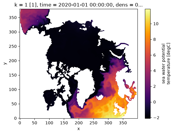
Surface temperature on the native curvilinear grid:
ds["temp"].isel(time=0, k=0).plot(cmap="inferno", center=False)
<matplotlib.collections.QuadMesh at 0x14d83d3ef230>
Regrid onto a GLORYS grid#
GLORYS ships a regular lon/lat/depth grid with a land mask. Pass it straight to regrid as target= — lon/lat/depth and the mask come from it.
GRIDS = "/nird/datapeak/NS9481K/MERCATOR_DATA/REGULAR_GRID_COORD"
glorys = xr.open_dataset(f"{GRIDS}/GLO-MFC_001_030_mask_bathy.nc")
glorys
<xarray.Dataset> Size: 511MB
Dimensions:     (depth: 50, latitude: 2041, longitude: 4320)
Coordinates:
  * depth       (depth) float32 200B 0.494 1.541 2.646 ... 5.275e+03 5.728e+03
  * latitude    (latitude) float32 8kB -80.0 -79.92 -79.83 ... 89.83 89.92 90.0
  * longitude   (longitude) float32 17kB -180.0 -179.9 -179.8 ... 179.8 179.9
Data variables:
    mask        (depth, latitude, longitude) int8 441MB ...
    deptho      (latitude, longitude) float32 35MB ...
    deptho_lev  (latitude, longitude) float32 35MB ...
Attributes:
    title:                Bathymetry and mask for product GLOBAL_MULTIYEAR_PH...
    references:           http://marine.copernicus.eu
    credit:               E.U. Copernicus Marine Service Information (CMEMS)
    licence:              http://marine.copernicus.eu/services-portfolio/serv...
    contact:              servicedesk.cmems@mercator-ocean.eu
    producer:             CMEMS - Global Monitoring and Forecasting Centre
    institution:          Mercator Ocean
    Conventions:          CF-1.6
    area:                 GLOBAL
    source:               GLORYS12V1
product_user_manual: http://marine.copernicus.eu/documents/PUM/CMEMS-GLO...- depth: 50
- latitude: 2041
- longitude: 4320
- depth(depth)float320.494 1.541 ... 5.275e+03 5.728e+03
- units :
- m
- positive :
- down
- standard_name :
- depth
- axis :
- Z
array([4.940250e-01, 1.541375e+00, 2.645669e+00, 3.819495e+00, 5.078224e+00, 6.440614e+00, 7.929560e+00, 9.572997e+00, 1.140500e+01, 1.346714e+01, 1.581007e+01, 1.849556e+01, 2.159882e+01, 2.521141e+01, 2.944473e+01, 3.443415e+01, 4.034405e+01, 4.737369e+01, 5.576429e+01, 6.580727e+01, 7.785385e+01, 9.232607e+01, 1.097293e+02, 1.306660e+02, 1.558507e+02, 1.861256e+02, 2.224752e+02, 2.660403e+02, 3.181274e+02, 3.802130e+02, 4.539377e+02, 5.410889e+02, 6.435668e+02, 7.633331e+02, 9.023393e+02, 1.062440e+03, 1.245291e+03, 1.452251e+03, 1.684284e+03, 1.941893e+03, 2.225078e+03, 2.533336e+03, 2.865703e+03, 3.220820e+03, 3.597032e+03, 3.992484e+03, 4.405224e+03, 4.833291e+03, 5.274784e+03, 5.727917e+03], dtype=float32) - latitude(latitude)float32-80.0 -79.92 -79.83 ... 89.92 90.0
- step :
- 0.083333336
- units :
- degrees_north
- standard_name :
- latitude
- axis :
- Y
array([-80. , -79.916664, -79.833336, ..., 89.833336, 89.916664, 90. ], shape=(2041,), dtype=float32) - longitude(longitude)float32-180.0 -179.9 ... 179.8 179.9
- step :
- 0.083333336
- units :
- degrees_east
- standard_name :
- longitude
- axis :
- X
array([-180.     , -179.91667, -179.83333, ...,  179.75   ,  179.83333,
        179.91667], shape=(4320,), dtype=float32)
- mask(depth, latitude, longitude)int8...
- long_name :
- Land-sea mask: 1 = sea ; 0 = land
- standard_name :
- sea_binary_mask
- units :
- 1
[440856000 values with dtype=int8]
- deptho(latitude, longitude)float32...
- long_name :
- Bathymetry
- standard_name :
- sea_floor_depth_below_geoid
- units :
- m
[8817120 values with dtype=float32]
- deptho_lev(latitude, longitude)float32...
- long_name :
- Model level number at sea floor
- standard_name :
- model_level_number_at_sea_floor
- units :
- 1
[8817120 values with dtype=float32]
- title :
- Bathymetry and mask for product GLOBAL_MULTIYEAR_PHY_001_030
- references :
- http://marine.copernicus.eu
- credit :
- E.U. Copernicus Marine Service Information (CMEMS)
- licence :
- http://marine.copernicus.eu/services-portfolio/service-commitments-and-licence/
- contact :
- servicedesk.cmems@mercator-ocean.eu
- producer :
- CMEMS - Global Monitoring and Forecasting Centre
- institution :
- Mercator Ocean
- Conventions :
- CF-1.6
- area :
- GLOBAL
- source :
- GLORYS12V1
- product_user_manual :
- http://marine.copernicus.eu/documents/PUM/CMEMS-GLO-PUM-001-030.pdf
# Conservative horizontal + vertical, in one call, onto the GLORYS grid.
%time ds_g = xhycom.regrid(ds, target=glorys, grid=grid)
CPU times: user 55.1 s, sys: 2.01 s, total: 57.2 s
Wall time: 57.9 s
This operation was slow: it computes the xESMF weight matrix that maps the HYCOM grid onto the GLORYS grid. The regridding itself is lazy — regrid returns dask-backed fields and the actual remap is deferred until you load them — so the time above is essentially all weight generation. Those weights depend only on the source and target grids, not on the field values or the time step, so the cost is the same whether you regrid a single slice or a whole year. That also means they can be built once and reused, which is done in the Caching the regrid weights section below.
ds_g # repr shows dask chunks — nothing computed yet
<xarray.Dataset> Size: 52TB
Dimensions:     (time: 366, lat: 624, lon: 4320, depth: 50, ki: 51)
Coordinates:
  * time        (time) object 3kB 2020-01-01 00:00:00 ... 2020-12-31 00:00:00
  * lat         (lat) float32 2kB 38.08 38.17 38.25 38.33 ... 89.83 89.92 90.0
  * lon         (lon) float32 17kB -180.0 -179.9 -179.8 ... 179.8 179.8 179.9
  * depth       (depth) float64 400B 0.494 1.541 2.646 ... 5.275e+03 5.728e+03
  * ki          (ki) int64 408B 0 1 2 3 4 5 6 7 8 ... 42 43 44 45 46 47 48 49 50
Data variables: (12/82)
    montg1      (time, lat, lon, depth) float64 395GB dask.array<chunksize=(1, 624, 4320, 50), meta=np.ndarray>
    srfhgt      (time, lat, lon, depth) float64 395GB dask.array<chunksize=(1, 624, 4320, 50), meta=np.ndarray>
    oneta       (time, lat, lon, depth) float64 395GB dask.array<chunksize=(1, 624, 4320, 50), meta=np.ndarray>
    surflx      (time, lat, lon, depth) float64 395GB dask.array<chunksize=(1, 624, 4320, 50), meta=np.ndarray>
    wtrflx      (time, lat, lon, depth) float64 395GB dask.array<chunksize=(1, 624, 4320, 50), meta=np.ndarray>
    salflx      (time, lat, lon, depth) float64 395GB dask.array<chunksize=(1, 624, 4320, 50), meta=np.ndarray>
    ...          ...
    light_sw    (time, lat, lon, depth) float64 395GB dask.array<chunksize=(1, 624, 4320, 50), meta=np.ndarray>
    attenuat    (time, lat, lon, depth) float64 395GB dask.array<chunksize=(1, 624, 4320, 50), meta=np.ndarray>
    total_ch    (time, lat, lon, depth) float64 395GB dask.array<chunksize=(1, 624, 4320, 50), meta=np.ndarray>
    total_ca    (time, lat, lon, depth) float64 395GB dask.array<chunksize=(1, 624, 4320, 50), meta=np.ndarray>
    u-vel.      (time, lat, lon, depth) float64 395GB dask.array<chunksize=(1, 624, 4320, 50), meta=np.ndarray>
    v-vel.      (time, lat, lon, depth) float64 395GB dask.array<chunksize=(1, 624, 4320, 50), meta=np.ndarray>
Attributes:
    iversn:         23
    iexpt:          28
    yrflag:         3
    archive_type:   mean
regrid_method: conservative- time: 366
- lat: 624
- lon: 4320
- depth: 50
- ki: 51
- time(time)object2020-01-01 00:00:00 ... 2020-12-...
- long_name :
- time
- axis :
- T
array([cftime.DatetimeGregorian(2020, 1, 1, 0, 0, 0, 0, has_year_zero=False), cftime.DatetimeGregorian(2020, 1, 2, 0, 0, 0, 0, has_year_zero=False), cftime.DatetimeGregorian(2020, 1, 3, 0, 0, 0, 0, has_year_zero=False), ..., cftime.DatetimeGregorian(2020, 12, 29, 0, 0, 0, 0, has_year_zero=False), cftime.DatetimeGregorian(2020, 12, 30, 0, 0, 0, 0, has_year_zero=False), cftime.DatetimeGregorian(2020, 12, 31, 0, 0, 0, 0, has_year_zero=False)], shape=(366,), dtype=object) - lat(lat)float3238.08 38.17 38.25 ... 89.92 90.0
- standard_name :
- latitude
- units :
- degrees_north
array([38.083332, 38.166668, 38.25 , ..., 89.833336, 89.916664, 90. ], shape=(624,), dtype=float32) - lon(lon)float32-180.0 -179.9 ... 179.8 179.9
- standard_name :
- longitude
- units :
- degrees_east
array([-180. , -179.91667, -179.83333, ..., 179.75 , 179.83333, 179.91667], shape=(4320,), dtype=float32) - depth(depth)float640.494 1.541 ... 5.275e+03 5.728e+03
- long_name :
- depth
- units :
- m
- positive :
- down
- axis :
- Z
array([4.940250e-01, 1.541375e+00, 2.645669e+00, 3.819495e+00, 5.078224e+00, 6.440614e+00, 7.929560e+00, 9.572997e+00, 1.140500e+01, 1.346714e+01, 1.581007e+01, 1.849556e+01, 2.159882e+01, 2.521141e+01, 2.944473e+01, 3.443415e+01, 4.034405e+01, 4.737369e+01, 5.576429e+01, 6.580727e+01, 7.785385e+01, 9.232607e+01, 1.097293e+02, 1.306660e+02, 1.558507e+02, 1.861256e+02, 2.224752e+02, 2.660403e+02, 3.181274e+02, 3.802130e+02, 4.539377e+02, 5.410889e+02, 6.435668e+02, 7.633331e+02, 9.023393e+02, 1.062440e+03, 1.245291e+03, 1.452251e+03, 1.684284e+03, 1.941893e+03, 2.225078e+03, 2.533336e+03, 2.865703e+03, 3.220820e+03, 3.597032e+03, 3.992484e+03, 4.405224e+03, 4.833291e+03, 5.274784e+03, 5.727917e+03]) - ki(ki)int640 1 2 3 4 5 6 ... 45 46 47 48 49 50
- long_name :
- layer interface index
- units :
- 1
- axis :
- Z
array([ 0,  1,  2,  3,  4,  5,  6,  7,  8,  9, 10, 11, 12, 13, 14, 15, 16, 17,
       18, 19, 20, 21, 22, 23, 24, 25, 26, 27, 28, 29, 30, 31, 32, 33, 34, 35,
       36, 37, 38, 39, 40, 41, 42, 43, 44, 45, 46, 47, 48, 49, 50])
- montg1(time, lat, lon, depth)float64dask.array<chunksize=(1, 624, 4320, 50), meta=np.ndarray>
- long_name :
- Montgomery potential
- units :
- m2 s-2
Array Chunk Bytes 367.54 GiB 1.00 GiB Shape (366, 624, 4320, 50) (1, 624, 4320, 50) Dask graph 366 chunks in 743 graph layers Data type float64 numpy.ndarray - srfhgt(time, lat, lon, depth)float64dask.array<chunksize=(1, 624, 4320, 50), meta=np.ndarray>
- long_name :
- sea surface height
- units :
- m
- comment :
- converted from Pa (factor 0.101978)
Array Chunk Bytes 367.54 GiB 1.00 GiB Shape (366, 624, 4320, 50) (1, 624, 4320, 50) Dask graph 366 chunks in 744 graph layers Data type float64 numpy.ndarray - oneta(time, lat, lon, depth)float64dask.array<chunksize=(1, 624, 4320, 50), meta=np.ndarray>
- long_name :
- free surface elevation
- units :
- m
Array Chunk Bytes 367.54 GiB 1.00 GiB Shape (366, 624, 4320, 50) (1, 624, 4320, 50) Dask graph 366 chunks in 743 graph layers Data type float64 numpy.ndarray - surflx(time, lat, lon, depth)float64dask.array<chunksize=(1, 624, 4320, 50), meta=np.ndarray>
- long_name :
- net surface heat flux
- units :
- W m-2
Array Chunk Bytes 367.54 GiB 1.00 GiB Shape (366, 624, 4320, 50) (1, 624, 4320, 50) Dask graph 366 chunks in 743 graph layers Data type float64 numpy.ndarray - wtrflx(time, lat, lon, depth)float64dask.array<chunksize=(1, 624, 4320, 50), meta=np.ndarray>
- long_name :
- net surface freshwater flux
- units :
- m s-1
Array Chunk Bytes 367.54 GiB 1.00 GiB Shape (366, 624, 4320, 50) (1, 624, 4320, 50) Dask graph 366 chunks in 743 graph layers Data type float64 numpy.ndarray - salflx(time, lat, lon, depth)float64dask.array<chunksize=(1, 624, 4320, 50), meta=np.ndarray>
- long_name :
- surface salt flux
- units :
- PSU m s-1
Array Chunk Bytes 367.54 GiB 1.00 GiB Shape (366, 624, 4320, 50) (1, 624, 4320, 50) Dask graph 366 chunks in 743 graph layers Data type float64 numpy.ndarray - bl_dpth(time, lat, lon, depth)float64dask.array<chunksize=(1, 624, 4320, 50), meta=np.ndarray>
- long_name :
- boundary layer depth
- units :
- m
- comment :
- converted from Pa (factor 0.000101978)
Array Chunk Bytes 367.54 GiB 1.00 GiB Shape (366, 624, 4320, 50) (1, 624, 4320, 50) Dask graph 366 chunks in 744 graph layers Data type float64 numpy.ndarray - mix_dpth(time, lat, lon, depth)float64dask.array<chunksize=(1, 624, 4320, 50), meta=np.ndarray>
- long_name :
- mixed layer depth
- units :
- m
- comment :
- converted from Pa (factor 0.000101978)
Array Chunk Bytes 367.54 GiB 1.00 GiB Shape (366, 624, 4320, 50) (1, 624, 4320, 50) Dask graph 366 chunks in 744 graph layers Data type float64 numpy.ndarray - tmix(time, lat, lon, depth)float64dask.array<chunksize=(1, 624, 4320, 50), meta=np.ndarray>
- long_name :
- mixed layer temperature
- units :
- degC
Array Chunk Bytes 367.54 GiB 1.00 GiB Shape (366, 624, 4320, 50) (1, 624, 4320, 50) Dask graph 366 chunks in 743 graph layers Data type float64 numpy.ndarray - smix(time, lat, lon, depth)float64dask.array<chunksize=(1, 624, 4320, 50), meta=np.ndarray>
- long_name :
- mixed layer salinity
- units :
- PSU
Array Chunk Bytes 367.54 GiB 1.00 GiB Shape (366, 624, 4320, 50) (1, 624, 4320, 50) Dask graph 366 chunks in 743 graph layers Data type float64 numpy.ndarray - thmix(time, lat, lon, depth)float64dask.array<chunksize=(1, 624, 4320, 50), meta=np.ndarray>
- long_name :
- mixed layer thickness
- units :
- m
- comment :
- converted from Pa (factor 0.000101978)
Array Chunk Bytes 367.54 GiB 1.00 GiB Shape (366, 624, 4320, 50) (1, 624, 4320, 50) Dask graph 366 chunks in 744 graph layers Data type float64 numpy.ndarray - kemix(time, lat, lon, depth)float64dask.array<chunksize=(1, 624, 4320, 50), meta=np.ndarray>
- long_name :
- mixed layer kinetic energy
- units :
- m2 s-2
Array Chunk Bytes 367.54 GiB 1.00 GiB Shape (366, 624, 4320, 50) (1, 624, 4320, 50) Dask graph 366 chunks in 743 graph layers Data type float64 numpy.ndarray - covice(time, lat, lon, depth)float64dask.array<chunksize=(1, 624, 4320, 50), meta=np.ndarray>
- long_name :
- sea ice coverage fraction
- units :
- 1
Array Chunk Bytes 367.54 GiB 1.00 GiB Shape (366, 624, 4320, 50) (1, 624, 4320, 50) Dask graph 366 chunks in 743 graph layers Data type float64 numpy.ndarray - thkice(time, lat, lon, depth)float64dask.array<chunksize=(1, 624, 4320, 50), meta=np.ndarray>
- long_name :
- sea ice thickness
- units :
- m
Array Chunk Bytes 367.54 GiB 1.00 GiB Shape (366, 624, 4320, 50) (1, 624, 4320, 50) Dask graph 366 chunks in 743 graph layers Data type float64 numpy.ndarray - temice(time, lat, lon, depth)float64dask.array<chunksize=(1, 624, 4320, 50), meta=np.ndarray>
- long_name :
- sea ice surface temperature
- units :
- degC
Array Chunk Bytes 367.54 GiB 1.00 GiB Shape (366, 624, 4320, 50) (1, 624, 4320, 50) Dask graph 366 chunks in 743 graph layers Data type float64 numpy.ndarray - kebtrop(time, lat, lon, depth)float64dask.array<chunksize=(1, 624, 4320, 50), meta=np.ndarray>
- long_name :
- barotropic kinetic energy
- units :
- m2 s-2
Array Chunk Bytes 367.54 GiB 1.00 GiB Shape (366, 624, 4320, 50) (1, 624, 4320, 50) Dask graph 366 chunks in 743 graph layers Data type float64 numpy.ndarray - light_pa(time, ki, lat, lon, depth)float64dask.array<chunksize=(1, 51, 624, 4320, 50), meta=np.ndarray>
- long_name :
- PAR irradiance
- units :
- W m-2
Array Chunk Bytes 18.31 TiB 51.22 GiB Shape (366, 51, 624, 4320, 50) (1, 51, 624, 4320, 50) Dask graph 366 chunks in 743 graph layers Data type float64 numpy.ndarray - ECO_sed4(time, lat, lon, depth)float64dask.array<chunksize=(1, 624, 4320, 50), meta=np.ndarray>
- long_name :
- sediment pool 4
- units :
- mmol m-2
Array Chunk Bytes 367.54 GiB 1.00 GiB Shape (366, 624, 4320, 50) (1, 624, 4320, 50) Dask graph 366 chunks in 743 graph layers Data type float64 numpy.ndarray - ECO_sed1(time, lat, lon, depth)float64dask.array<chunksize=(1, 624, 4320, 50), meta=np.ndarray>
- long_name :
- sediment pool 1
- units :
- mmol m-2
Array Chunk Bytes 367.54 GiB 1.00 GiB Shape (366, 624, 4320, 50) (1, 624, 4320, 50) Dask graph 366 chunks in 743 graph layers Data type float64 numpy.ndarray - ECO_sed2(time, lat, lon, depth)float64dask.array<chunksize=(1, 624, 4320, 50), meta=np.ndarray>
- long_name :
- sediment pool 2
- units :
- mmol m-2
Array Chunk Bytes 367.54 GiB 1.00 GiB Shape (366, 624, 4320, 50) (1, 624, 4320, 50) Dask graph 366 chunks in 743 graph layers Data type float64 numpy.ndarray - ECO_sed3(time, lat, lon, depth)float64dask.array<chunksize=(1, 624, 4320, 50), meta=np.ndarray>
- long_name :
- sediment pool 3
- units :
- mmol m-2
Array Chunk Bytes 367.54 GiB 1.00 GiB Shape (366, 624, 4320, 50) (1, 624, 4320, 50) Dask graph 366 chunks in 743 graph layers Data type float64 numpy.ndarray - CO2_fair(time, lat, lon, depth)float64dask.array<chunksize=(1, 624, 4320, 50), meta=np.ndarray>
- long_name :
- air-sea CO2 flux
- units :
- mmol C m-2 d-1
Array Chunk Bytes 367.54 GiB 1.00 GiB Shape (366, 624, 4320, 50) (1, 624, 4320, 50) Dask graph 366 chunks in 743 graph layers Data type float64 numpy.ndarray - CO2_wind(time, lat, lon, depth)float64dask.array<chunksize=(1, 624, 4320, 50), meta=np.ndarray>
- long_name :
- wind speed for gas exchange
- units :
- m s-1
Array Chunk Bytes 367.54 GiB 1.00 GiB Shape (366, 624, 4320, 50) (1, 624, 4320, 50) Dask graph 366 chunks in 743 graph layers Data type float64 numpy.ndarray - ECO_bots(time, lat, lon, depth)float64dask.array<chunksize=(1, 624, 4320, 50), meta=np.ndarray>
- long_name :
- bottom sediment flux
- units :
- 1
Array Chunk Bytes 367.54 GiB 1.00 GiB Shape (366, 624, 4320, 50) (1, 624, 4320, 50) Dask graph 366 chunks in 743 graph layers Data type float64 numpy.ndarray - surface__1(time, lat, lon, depth)float64dask.array<chunksize=(1, 624, 4320, 50), meta=np.ndarray>
Array Chunk Bytes 367.54 GiB 1.00 GiB Shape (366, 624, 4320, 50) (1, 624, 4320, 50) Dask graph 366 chunks in 743 graph layers Data type float64 numpy.ndarray - surface__2(time, lat, lon, depth)float64dask.array<chunksize=(1, 624, 4320, 50), meta=np.ndarray>
Array Chunk Bytes 367.54 GiB 1.00 GiB Shape (366, 624, 4320, 50) (1, 624, 4320, 50) Dask graph 366 chunks in 743 graph layers Data type float64 numpy.ndarray - u_btrop(time, lat, lon, depth)float64dask.array<chunksize=(1, 624, 4320, 50), meta=np.ndarray>
- long_name :
- eastward component of barotropic x velocity
- units :
- m s-1
- standard_name :
- eastward_sea_water_velocity
- comment :
- de-staggered to T-points and rotated to geographic axes
Array Chunk Bytes 367.54 GiB 1.00 GiB Shape (366, 624, 4320, 50) (1, 624, 4320, 50) Dask graph 366 chunks in 1494 graph layers Data type float64 numpy.ndarray - v_btrop(time, lat, lon, depth)float64dask.array<chunksize=(1, 624, 4320, 50), meta=np.ndarray>
- long_name :
- northward component of barotropic y velocity
- units :
- m s-1
- standard_name :
- northward_sea_water_velocity
- comment :
- de-staggered to T-points and rotated to geographic axes
Array Chunk Bytes 367.54 GiB 1.00 GiB Shape (366, 624, 4320, 50) (1, 624, 4320, 50) Dask graph 366 chunks in 1494 graph layers Data type float64 numpy.ndarray - umix(time, lat, lon, depth)float64dask.array<chunksize=(1, 624, 4320, 50), meta=np.ndarray>
- long_name :
- eastward component of mixed layer x velocity
- units :
- m s-1
- standard_name :
- eastward_sea_water_velocity
- comment :
- de-staggered to T-points and rotated to geographic axes
Array Chunk Bytes 367.54 GiB 1.00 GiB Shape (366, 624, 4320, 50) (1, 624, 4320, 50) Dask graph 366 chunks in 1494 graph layers Data type float64 numpy.ndarray - vmix(time, lat, lon, depth)float64dask.array<chunksize=(1, 624, 4320, 50), meta=np.ndarray>
- long_name :
- northward component of mixed layer y velocity
- units :
- m s-1
- standard_name :
- northward_sea_water_velocity
- comment :
- de-staggered to T-points and rotated to geographic axes
Array Chunk Bytes 367.54 GiB 1.00 GiB Shape (366, 624, 4320, 50) (1, 624, 4320, 50) Dask graph 366 chunks in 1494 graph layers Data type float64 numpy.ndarray - si_u(time, lat, lon, depth)float64dask.array<chunksize=(1, 624, 4320, 50), meta=np.ndarray>
- long_name :
- eastward component of sea ice x velocity
- units :
- m s-1
- standard_name :
- eastward_sea_water_velocity
- comment :
- de-staggered to T-points and rotated to geographic axes
Array Chunk Bytes 367.54 GiB 1.00 GiB Shape (366, 624, 4320, 50) (1, 624, 4320, 50) Dask graph 366 chunks in 1494 graph layers Data type float64 numpy.ndarray - si_v(time, lat, lon, depth)float64dask.array<chunksize=(1, 624, 4320, 50), meta=np.ndarray>
- long_name :
- northward component of sea ice y velocity
- units :
- m s-1
- standard_name :
- northward_sea_water_velocity
- comment :
- de-staggered to T-points and rotated to geographic axes
Array Chunk Bytes 367.54 GiB 1.00 GiB Shape (366, 624, 4320, 50) (1, 624, 4320, 50) Dask graph 366 chunks in 1494 graph layers Data type float64 numpy.ndarray - k.e.(time, lat, lon, depth)float64dask.array<chunksize=(1, 624, 4320, 50), meta=np.ndarray>
- long_name :
- kinetic energy
- units :
- m2 s-2
Array Chunk Bytes 367.54 GiB 1.00 GiB Shape (366, 624, 4320, 50) (1, 624, 4320, 50) Dask graph 366 chunks in 1505 graph layers Data type float64 numpy.ndarray - temp(time, lat, lon, depth)float64dask.array<chunksize=(1, 624, 4320, 50), meta=np.ndarray>
- long_name :
- sea water potential temperature
- units :
- degC
Array Chunk Bytes 367.54 GiB 1.00 GiB Shape (366, 624, 4320, 50) (1, 624, 4320, 50) Dask graph 366 chunks in 1505 graph layers Data type float64 numpy.ndarray - salin(time, lat, lon, depth)float64dask.array<chunksize=(1, 624, 4320, 50), meta=np.ndarray>
- long_name :
- sea water salinity
- units :
- PSU
Array Chunk Bytes 367.54 GiB 1.00 GiB Shape (366, 624, 4320, 50) (1, 624, 4320, 50) Dask graph 366 chunks in 1505 graph layers Data type float64 numpy.ndarray - density(time, lat, lon, depth)float64dask.array<chunksize=(1, 624, 4320, 50), meta=np.ndarray>
- long_name :
- sea water potential density (sigma-2)
- units :
- kg m-3
Array Chunk Bytes 367.54 GiB 1.00 GiB Shape (366, 624, 4320, 50) (1, 624, 4320, 50) Dask graph 366 chunks in 1505 graph layers Data type float64 numpy.ndarray - CO2_c(time, lat, lon, depth)float64dask.array<chunksize=(1, 624, 4320, 50), meta=np.ndarray>
- long_name :
- dissolved inorganic carbon
- units :
- mmol C m-3
Array Chunk Bytes 367.54 GiB 1.00 GiB Shape (366, 624, 4320, 50) (1, 624, 4320, 50) Dask graph 366 chunks in 1505 graph layers Data type float64 numpy.ndarray - CO2_TA(time, lat, lon, depth)float64dask.array<chunksize=(1, 624, 4320, 50), meta=np.ndarray>
- long_name :
- total alkalinity
- units :
- mmol eq m-3
Array Chunk Bytes 367.54 GiB 1.00 GiB Shape (366, 624, 4320, 50) (1, 624, 4320, 50) Dask graph 366 chunks in 1505 graph layers Data type float64 numpy.ndarray - ECO_no3(time, lat, lon, depth)float64dask.array<chunksize=(1, 624, 4320, 50), meta=np.ndarray>
- long_name :
- nitrate
- units :
- mmol N m-3
Array Chunk Bytes 367.54 GiB 1.00 GiB Shape (366, 624, 4320, 50) (1, 624, 4320, 50) Dask graph 366 chunks in 1505 graph layers Data type float64 numpy.ndarray - ECO_nh4(time, lat, lon, depth)float64dask.array<chunksize=(1, 624, 4320, 50), meta=np.ndarray>
- long_name :
- ammonium
- units :
- mmol N m-3
Array Chunk Bytes 367.54 GiB 1.00 GiB Shape (366, 624, 4320, 50) (1, 624, 4320, 50) Dask graph 366 chunks in 1505 graph layers Data type float64 numpy.ndarray - ECO_pho(time, lat, lon, depth)float64dask.array<chunksize=(1, 624, 4320, 50), meta=np.ndarray>
- long_name :
- phosphate
- units :
- mmol P m-3
Array Chunk Bytes 367.54 GiB 1.00 GiB Shape (366, 624, 4320, 50) (1, 624, 4320, 50) Dask graph 366 chunks in 1505 graph layers Data type float64 numpy.ndarray - ECO_sil(time, lat, lon, depth)float64dask.array<chunksize=(1, 624, 4320, 50), meta=np.ndarray>
- long_name :
- silicate
- units :
- mmol Si m-3
Array Chunk Bytes 367.54 GiB 1.00 GiB Shape (366, 624, 4320, 50) (1, 624, 4320, 50) Dask graph 366 chunks in 1505 graph layers Data type float64 numpy.ndarray - ECO_oxy(time, lat, lon, depth)float64dask.array<chunksize=(1, 624, 4320, 50), meta=np.ndarray>
- long_name :
- dissolved oxygen
- units :
- mmol O m-3
Array Chunk Bytes 367.54 GiB 1.00 GiB Shape (366, 624, 4320, 50) (1, 624, 4320, 50) Dask graph 366 chunks in 1505 graph layers Data type float64 numpy.ndarray - ECO_fla(time, lat, lon, depth)float64dask.array<chunksize=(1, 624, 4320, 50), meta=np.ndarray>
- long_name :
- flagellate carbon
- units :
- mmol C m-3
Array Chunk Bytes 367.54 GiB 1.00 GiB Shape (366, 624, 4320, 50) (1, 624, 4320, 50) Dask graph 366 chunks in 1505 graph layers Data type float64 numpy.ndarray - ECO_dia(time, lat, lon, depth)float64dask.array<chunksize=(1, 624, 4320, 50), meta=np.ndarray>
- long_name :
- diatom carbon
- units :
- mmol C m-3
Array Chunk Bytes 367.54 GiB 1.00 GiB Shape (366, 624, 4320, 50) (1, 624, 4320, 50) Dask graph 366 chunks in 1505 graph layers Data type float64 numpy.ndarray - ECO_ccl(time, lat, lon, depth)float64dask.array<chunksize=(1, 624, 4320, 50), meta=np.ndarray>
- long_name :
- coccolithophore carbon
- units :
- mmol C m-3
Array Chunk Bytes 367.54 GiB 1.00 GiB Shape (366, 624, 4320, 50) (1, 624, 4320, 50) Dask graph 366 chunks in 1505 graph layers Data type float64 numpy.ndarray - ECO_cclc(time, lat, lon, depth)float64dask.array<chunksize=(1, 624, 4320, 50), meta=np.ndarray>
- long_name :
- coccolithophore calcite carbon
- units :
- mmol C m-3
Array Chunk Bytes 367.54 GiB 1.00 GiB Shape (366, 624, 4320, 50) (1, 624, 4320, 50) Dask graph 366 chunks in 1505 graph layers Data type float64 numpy.ndarray - ECO_caco(time, lat, lon, depth)float64dask.array<chunksize=(1, 624, 4320, 50), meta=np.ndarray>
- long_name :
- particulate inorganic carbon (calcite)
- units :
- mmol C m-3
Array Chunk Bytes 367.54 GiB 1.00 GiB Shape (366, 624, 4320, 50) (1, 624, 4320, 50) Dask graph 366 chunks in 1505 graph layers Data type float64 numpy.ndarray - ECO_diac(time, lat, lon, depth)float64dask.array<chunksize=(1, 624, 4320, 50), meta=np.ndarray>
- long_name :
- diatom calcite carbon
- units :
- mmol C m-3
Array Chunk Bytes 367.54 GiB 1.00 GiB Shape (366, 624, 4320, 50) (1, 624, 4320, 50) Dask graph 366 chunks in 1505 graph layers Data type float64 numpy.ndarray - ECO_flac(time, lat, lon, depth)float64dask.array<chunksize=(1, 624, 4320, 50), meta=np.ndarray>
- long_name :
- flagellate calcite carbon
- units :
- mmol C m-3
Array Chunk Bytes 367.54 GiB 1.00 GiB Shape (366, 624, 4320, 50) (1, 624, 4320, 50) Dask graph 366 chunks in 1505 graph layers Data type float64 numpy.ndarray - ECO_micr(time, lat, lon, depth)float64dask.array<chunksize=(1, 624, 4320, 50), meta=np.ndarray>
- long_name :
- microzooplankton carbon
- units :
- mmol C m-3
Array Chunk Bytes 367.54 GiB 1.00 GiB Shape (366, 624, 4320, 50) (1, 624, 4320, 50) Dask graph 366 chunks in 1505 graph layers Data type float64 numpy.ndarray - ECO_meso(time, lat, lon, depth)float64dask.array<chunksize=(1, 624, 4320, 50), meta=np.ndarray>
- long_name :
- mesozooplankton carbon
- units :
- mmol C m-3
Array Chunk Bytes 367.54 GiB 1.00 GiB Shape (366, 624, 4320, 50) (1, 624, 4320, 50) Dask graph 366 chunks in 1505 graph layers Data type float64 numpy.ndarray - ECO_det(time, lat, lon, depth)float64dask.array<chunksize=(1, 624, 4320, 50), meta=np.ndarray>
- long_name :
- detritus carbon
- units :
- mmol C m-3
Array Chunk Bytes 367.54 GiB 1.00 GiB Shape (366, 624, 4320, 50) (1, 624, 4320, 50) Dask graph 366 chunks in 1505 graph layers Data type float64 numpy.ndarray - ECO_opa(time, lat, lon, depth)float64dask.array<chunksize=(1, 624, 4320, 50), meta=np.ndarray>
- long_name :
- opal (biogenic silica)
- units :
- mmol Si m-3
Array Chunk Bytes 367.54 GiB 1.00 GiB Shape (366, 624, 4320, 50) (1, 624, 4320, 50) Dask graph 366 chunks in 1505 graph layers Data type float64 numpy.ndarray - ECO_dom(time, lat, lon, depth)float64dask.array<chunksize=(1, 624, 4320, 50), meta=np.ndarray>
- long_name :
- dissolved organic matter carbon
- units :
- mmol C m-3
Array Chunk Bytes 367.54 GiB 1.00 GiB Shape (366, 624, 4320, 50) (1, 624, 4320, 50) Dask graph 366 chunks in 1505 graph layers Data type float64 numpy.ndarray - ECO_dsnk(time, lat, lon, depth)float64dask.array<chunksize=(1, 624, 4320, 50), meta=np.ndarray>
- long_name :
- detritus sinking flux
- units :
- mmol C m-2 s-1
Array Chunk Bytes 367.54 GiB 1.00 GiB Shape (366, 624, 4320, 50) (1, 624, 4320, 50) Dask graph 366 chunks in 1505 graph layers Data type float64 numpy.ndarray - CO2_pH(time, lat, lon, depth)float64dask.array<chunksize=(1, 624, 4320, 50), meta=np.ndarray>
- long_name :
- seawater pH
- units :
- 1
Array Chunk Bytes 367.54 GiB 1.00 GiB Shape (366, 624, 4320, 50) (1, 624, 4320, 50) Dask graph 366 chunks in 1505 graph layers Data type float64 numpy.ndarray - CO2_pCO2(time, lat, lon, depth)float64dask.array<chunksize=(1, 624, 4320, 50), meta=np.ndarray>
- long_name :
- partial pressure of CO2
- units :
- uatm
Array Chunk Bytes 367.54 GiB 1.00 GiB Shape (366, 624, 4320, 50) (1, 624, 4320, 50) Dask graph 366 chunks in 1505 graph layers Data type float64 numpy.ndarray - CO2_Carb_1(time, lat, lon, depth)float64dask.array<chunksize=(1, 624, 4320, 50), meta=np.ndarray>
- long_name :
- carbonate concentration
- units :
- mmol C m-3
Array Chunk Bytes 367.54 GiB 1.00 GiB Shape (366, 624, 4320, 50) (1, 624, 4320, 50) Dask graph 366 chunks in 1505 graph layers Data type float64 numpy.ndarray - CO2_BiCa(time, lat, lon, depth)float64dask.array<chunksize=(1, 624, 4320, 50), meta=np.ndarray>
- long_name :
- bicarbonate concentration
- units :
- mmol C m-3
Array Chunk Bytes 367.54 GiB 1.00 GiB Shape (366, 624, 4320, 50) (1, 624, 4320, 50) Dask graph 366 chunks in 1505 graph layers Data type float64 numpy.ndarray - CO2_Carb_2(time, lat, lon, depth)float64dask.array<chunksize=(1, 624, 4320, 50), meta=np.ndarray>
- long_name :
- carbonate concentration
- units :
- mmol C m-3
Array Chunk Bytes 367.54 GiB 1.00 GiB Shape (366, 624, 4320, 50) (1, 624, 4320, 50) Dask graph 366 chunks in 1505 graph layers Data type float64 numpy.ndarray - CO2_Om_c(time, lat, lon, depth)float64dask.array<chunksize=(1, 624, 4320, 50), meta=np.ndarray>
- long_name :
- calcite saturation state (Omega)
- units :
- 1
Array Chunk Bytes 367.54 GiB 1.00 GiB Shape (366, 624, 4320, 50) (1, 624, 4320, 50) Dask graph 366 chunks in 1505 graph layers Data type float64 numpy.ndarray - CO2_Om_a(time, lat, lon, depth)float64dask.array<chunksize=(1, 624, 4320, 50), meta=np.ndarray>
- long_name :
- aragonite saturation state (Omega)
- units :
- 1
Array Chunk Bytes 367.54 GiB 1.00 GiB Shape (366, 624, 4320, 50) (1, 624, 4320, 50) Dask graph 366 chunks in 1505 graph layers Data type float64 numpy.ndarray - ECO_prim(time, lat, lon, depth)float64dask.array<chunksize=(1, 624, 4320, 50), meta=np.ndarray>
- long_name :
- primary production
- units :
- mmol C m-3 s-1
Array Chunk Bytes 367.54 GiB 1.00 GiB Shape (366, 624, 4320, 50) (1, 624, 4320, 50) Dask graph 366 chunks in 1505 graph layers Data type float64 numpy.ndarray - ECO_secp(time, lat, lon, depth)float64dask.array<chunksize=(1, 624, 4320, 50), meta=np.ndarray>
- long_name :
- secondary production
- units :
- mmol C m-3 s-1
Array Chunk Bytes 367.54 GiB 1.00 GiB Shape (366, 624, 4320, 50) (1, 624, 4320, 50) Dask graph 366 chunks in 1505 graph layers Data type float64 numpy.ndarray - ECO_netp(time, lat, lon, depth)float64dask.array<chunksize=(1, 624, 4320, 50), meta=np.ndarray>
- long_name :
- net primary production
- units :
- mmol C m-3 s-1
Array Chunk Bytes 367.54 GiB 1.00 GiB Shape (366, 624, 4320, 50) (1, 624, 4320, 50) Dask graph 366 chunks in 1505 graph layers Data type float64 numpy.ndarray - ECO_parm(time, lat, lon, depth)float64dask.array<chunksize=(1, 624, 4320, 50), meta=np.ndarray>
- long_name :
- BGC parameter field
- units :
- 1
Array Chunk Bytes 367.54 GiB 1.00 GiB Shape (366, 624, 4320, 50) (1, 624, 4320, 50) Dask graph 366 chunks in 1505 graph layers Data type float64 numpy.ndarray - ECO_Nlim(time, lat, lon, depth)float64dask.array<chunksize=(1, 624, 4320, 50), meta=np.ndarray>
- long_name :
- nitrogen limitation factor
- units :
- 1
Array Chunk Bytes 367.54 GiB 1.00 GiB Shape (366, 624, 4320, 50) (1, 624, 4320, 50) Dask graph 366 chunks in 1505 graph layers Data type float64 numpy.ndarray - ECO_Plim(time, lat, lon, depth)float64dask.array<chunksize=(1, 624, 4320, 50), meta=np.ndarray>
- long_name :
- phosphorus limitation factor
- units :
- 1
Array Chunk Bytes 367.54 GiB 1.00 GiB Shape (366, 624, 4320, 50) (1, 624, 4320, 50) Dask graph 366 chunks in 1505 graph layers Data type float64 numpy.ndarray - ECO_Slim(time, lat, lon, depth)float64dask.array<chunksize=(1, 624, 4320, 50), meta=np.ndarray>
- long_name :
- silicate limitation factor
- units :
- 1
Array Chunk Bytes 367.54 GiB 1.00 GiB Shape (366, 624, 4320, 50) (1, 624, 4320, 50) Dask graph 366 chunks in 1505 graph layers Data type float64 numpy.ndarray - ECO_Llim(time, lat, lon, depth)float64dask.array<chunksize=(1, 624, 4320, 50), meta=np.ndarray>
- long_name :
- light limitation factor
- units :
- 1
Array Chunk Bytes 367.54 GiB 1.00 GiB Shape (366, 624, 4320, 50) (1, 624, 4320, 50) Dask graph 366 chunks in 1505 graph layers Data type float64 numpy.ndarray - ECO_deni(time, lat, lon, depth)float64dask.array<chunksize=(1, 624, 4320, 50), meta=np.ndarray>
- long_name :
- denitrification
- units :
- mmol N m-3 s-1
Array Chunk Bytes 367.54 GiB 1.00 GiB Shape (366, 624, 4320, 50) (1, 624, 4320, 50) Dask graph 366 chunks in 1505 graph layers Data type float64 numpy.ndarray - ECO_snks(time, lat, lon, depth)float64dask.array<chunksize=(1, 624, 4320, 50), meta=np.ndarray>
- long_name :
- sinking rate
- units :
- m d-1
Array Chunk Bytes 367.54 GiB 1.00 GiB Shape (366, 624, 4320, 50) (1, 624, 4320, 50) Dask graph 366 chunks in 1505 graph layers Data type float64 numpy.ndarray - ECO_c2ch_1(time, lat, lon, depth)float64dask.array<chunksize=(1, 624, 4320, 50), meta=np.ndarray>
- long_name :
- carbon to chlorophyll ratio
- units :
- g C g-1 Chl
Array Chunk Bytes 367.54 GiB 1.00 GiB Shape (366, 624, 4320, 50) (1, 624, 4320, 50) Dask graph 366 chunks in 1505 graph layers Data type float64 numpy.ndarray - ECO_c2ch_2(time, lat, lon, depth)float64dask.array<chunksize=(1, 624, 4320, 50), meta=np.ndarray>
- long_name :
- carbon to chlorophyll ratio
- units :
- g C g-1 Chl
Array Chunk Bytes 367.54 GiB 1.00 GiB Shape (366, 624, 4320, 50) (1, 624, 4320, 50) Dask graph 366 chunks in 1505 graph layers Data type float64 numpy.ndarray - ECO_c2ch_3(time, lat, lon, depth)float64dask.array<chunksize=(1, 624, 4320, 50), meta=np.ndarray>
- long_name :
- carbon to chlorophyll ratio
- units :
- g C g-1 Chl
Array Chunk Bytes 367.54 GiB 1.00 GiB Shape (366, 624, 4320, 50) (1, 624, 4320, 50) Dask graph 366 chunks in 1505 graph layers Data type float64 numpy.ndarray - light_sw(time, lat, lon, depth)float64dask.array<chunksize=(1, 624, 4320, 50), meta=np.ndarray>
- long_name :
- shortwave irradiance in water
- units :
- W m-2
Array Chunk Bytes 367.54 GiB 1.00 GiB Shape (366, 624, 4320, 50) (1, 624, 4320, 50) Dask graph 366 chunks in 1505 graph layers Data type float64 numpy.ndarray - attenuat(time, lat, lon, depth)float64dask.array<chunksize=(1, 624, 4320, 50), meta=np.ndarray>
- long_name :
- light attenuation coefficient
- units :
- m-1
Array Chunk Bytes 367.54 GiB 1.00 GiB Shape (366, 624, 4320, 50) (1, 624, 4320, 50) Dask graph 366 chunks in 1505 graph layers Data type float64 numpy.ndarray - total_ch(time, lat, lon, depth)float64dask.array<chunksize=(1, 624, 4320, 50), meta=np.ndarray>
- long_name :
- total chlorophyll
- units :
- mg Chl m-3
Array Chunk Bytes 367.54 GiB 1.00 GiB Shape (366, 624, 4320, 50) (1, 624, 4320, 50) Dask graph 366 chunks in 1505 graph layers Data type float64 numpy.ndarray - total_ca(time, lat, lon, depth)float64dask.array<chunksize=(1, 624, 4320, 50), meta=np.ndarray>
- long_name :
- total carbon
- units :
- mmol C m-3
Array Chunk Bytes 367.54 GiB 1.00 GiB Shape (366, 624, 4320, 50) (1, 624, 4320, 50) Dask graph 366 chunks in 1505 graph layers Data type float64 numpy.ndarray - u-vel.(time, lat, lon, depth)float64dask.array<chunksize=(1, 624, 4320, 50), meta=np.ndarray>
- long_name :
- eastward component of sea water x velocity
- units :
- m s-1
- hycom_velocity :
- total
- comment :
- de-staggered to T-points and rotated to geographic axes
- standard_name :
- eastward_sea_water_velocity
Array Chunk Bytes 367.54 GiB 1.00 GiB Shape (366, 624, 4320, 50) (1, 624, 4320, 50) Dask graph 366 chunks in 2256 graph layers Data type float64 numpy.ndarray - v-vel.(time, lat, lon, depth)float64dask.array<chunksize=(1, 624, 4320, 50), meta=np.ndarray>
- long_name :
- northward component of sea water y velocity
- units :
- m s-1
- hycom_velocity :
- total
- comment :
- de-staggered to T-points and rotated to geographic axes
- standard_name :
- northward_sea_water_velocity
Array Chunk Bytes 367.54 GiB 1.00 GiB Shape (366, 624, 4320, 50) (1, 624, 4320, 50) Dask graph 366 chunks in 2256 graph layers Data type float64 numpy.ndarray
- iversn :
- 23
- iexpt :
- 28
- yrflag :
- 3
- archive_type :
- mean
- regrid_method :
- conservative
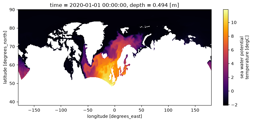
%time ds_g.temp.isel(time=0, depth=0).plot(figsize=(10, 4), cmap="inferno", center=False)
CPU times: user 8.47 s, sys: 1.1 s, total: 9.57 s
Wall time: 9.67 s
<matplotlib.collections.QuadMesh at 0x14d82be7e210>
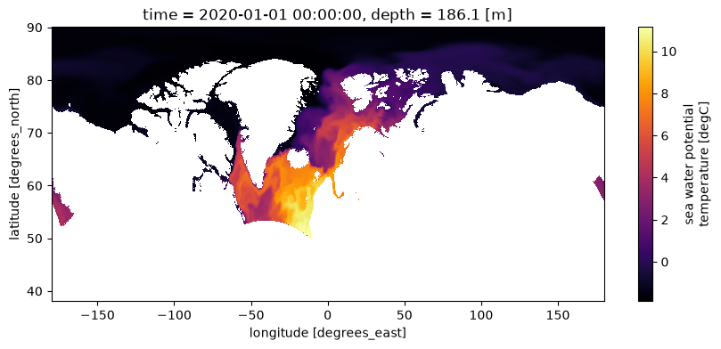
%time ds_g.temp.isel(time=0).sel(depth=200, method="nearest").plot(figsize=(10, 4), cmap="inferno", center=False)
CPU times: user 8.29 s, sys: 1.15 s, total: 9.44 s
Wall time: 9.5 s
<matplotlib.collections.QuadMesh at 0x14d82aec9e50>
Comparing to GLORYS#
With HYCOM on the GLORYS grid, a like-for-like comparison against the reanalysis is a straightforward subtraction — open a GLORYS field for the matching date and difference it.
# GLORYS reanalysis fields for the same date (thetao = potential temperature).
# Adjust the path / variable names to your GLORYS product if they differ.
glorys_data = xr.open_dataset(
    "/nird/datapeak/NS9481K/MERCATOR_DATA/PHY/2020/MERCATOR-PHY-24-2020-01-01-12.nc"
)
hycom_temp = ds_g["temp"].isel(time=0).sel(depth=250, method="nearest").compute()
glorys_temp = glorys_data["thetao"].isel(time=0).sel(depth=250, method="nearest").rename(longitude="lon", latitude="lat").compute()
vmin = hycom_temp.min().values
vmax = hycom_temp.max().values

fig, axs = plt.subplots(1, 3, figsize=(25, 3))

hycom_temp.plot(cmap="inferno", vmin=vmin, vmax=vmax, ax=axs[0])
glorys_temp.plot(cmap="inferno", vmin=vmin, vmax=vmax, ax=axs[1])
(hycom_temp - glorys_temp).plot()

for ax in axs:
    ax.set_ylim(50, None)      # latitude > 50

Custom target grid (arrays)#
Instead of a target= grid you can pass lon/lat/depth arrays directly:
lon = np.arange(-40, 40, 0.1)
lat = np.arange(55, 82, 0.1)
depth = np.array([0, 10, 20, 50, 100, 200, 500, 1000.0])
ds_box = xhycom.regrid(ds, lon=lon, lat=lat, depth=depth, grid=grid)
ds_box
<xarray.Dataset> Size: 305GB
Dimensions:     (time: 366, lat: 270, lon: 800, ki: 51, depth: 8)
Coordinates:
  * time        (time) object 3kB 2020-01-01 00:00:00 ... 2020-12-31 00:00:00
  * lat         (lat) float64 2kB 55.0 55.1 55.2 55.3 ... 81.6 81.7 81.8 81.9
  * lon         (lon) float64 6kB -40.0 -39.9 -39.8 -39.7 ... 39.7 39.8 39.9
  * ki          (ki) int64 408B 0 1 2 3 4 5 6 7 8 ... 42 43 44 45 46 47 48 49 50
  * depth       (depth) float64 64B 0.0 10.0 20.0 50.0 100.0 200.0 500.0 1e+03
Data variables: (12/82)
    montg1      (time, lat, lon) float64 632MB dask.array<chunksize=(1, 270, 800), meta=np.ndarray>
    srfhgt      (time, lat, lon) float64 632MB dask.array<chunksize=(1, 270, 800), meta=np.ndarray>
    oneta       (time, lat, lon) float64 632MB dask.array<chunksize=(1, 270, 800), meta=np.ndarray>
    surflx      (time, lat, lon) float64 632MB dask.array<chunksize=(1, 270, 800), meta=np.ndarray>
    wtrflx      (time, lat, lon) float64 632MB dask.array<chunksize=(1, 270, 800), meta=np.ndarray>
    salflx      (time, lat, lon) float64 632MB dask.array<chunksize=(1, 270, 800), meta=np.ndarray>
    ...          ...
    light_sw    (time, lat, lon, depth) float64 5GB dask.array<chunksize=(1, 270, 800, 8), meta=np.ndarray>
    attenuat    (time, lat, lon, depth) float64 5GB dask.array<chunksize=(1, 270, 800, 8), meta=np.ndarray>
    total_ch    (time, lat, lon, depth) float64 5GB dask.array<chunksize=(1, 270, 800, 8), meta=np.ndarray>
    total_ca    (time, lat, lon, depth) float64 5GB dask.array<chunksize=(1, 270, 800, 8), meta=np.ndarray>
    u-vel.      (time, lat, lon, depth) float64 5GB dask.array<chunksize=(1, 270, 800, 8), meta=np.ndarray>
    v-vel.      (time, lat, lon, depth) float64 5GB dask.array<chunksize=(1, 270, 800, 8), meta=np.ndarray>
Attributes:
    iversn:         23
    iexpt:          28
    yrflag:         3
    archive_type:   mean
regrid_method: conservative- time: 366
- lat: 270
- lon: 800
- ki: 51
- depth: 8
- time(time)object2020-01-01 00:00:00 ... 2020-12-...
- long_name :
- time
- axis :
- T
array([cftime.DatetimeGregorian(2020, 1, 1, 0, 0, 0, 0, has_year_zero=False), cftime.DatetimeGregorian(2020, 1, 2, 0, 0, 0, 0, has_year_zero=False), cftime.DatetimeGregorian(2020, 1, 3, 0, 0, 0, 0, has_year_zero=False), ..., cftime.DatetimeGregorian(2020, 12, 29, 0, 0, 0, 0, has_year_zero=False), cftime.DatetimeGregorian(2020, 12, 30, 0, 0, 0, 0, has_year_zero=False), cftime.DatetimeGregorian(2020, 12, 31, 0, 0, 0, 0, has_year_zero=False)], shape=(366,), dtype=object) - lat(lat)float6455.0 55.1 55.2 ... 81.7 81.8 81.9
- standard_name :
- latitude
- units :
- degrees_north
array([55. , 55.1, 55.2, ..., 81.7, 81.8, 81.9], shape=(270,))
- lon(lon)float64-40.0 -39.9 -39.8 ... 39.8 39.9
- standard_name :
- longitude
- units :
- degrees_east
array([-40. , -39.9, -39.8, ..., 39.7, 39.8, 39.9], shape=(800,))
- ki(ki)int640 1 2 3 4 5 6 ... 45 46 47 48 49 50
- long_name :
- layer interface index
- units :
- 1
- axis :
- Z
array([ 0, 1, 2, 3, 4, 5, 6, 7, 8, 9, 10, 11, 12, 13, 14, 15, 16, 17, 18, 19, 20, 21, 22, 23, 24, 25, 26, 27, 28, 29, 30, 31, 32, 33, 34, 35, 36, 37, 38, 39, 40, 41, 42, 43, 44, 45, 46, 47, 48, 49, 50]) - depth(depth)float640.0 10.0 20.0 ... 200.0 500.0 1e+03
- long_name :
- depth
- units :
- m
- positive :
- down
- axis :
- Z
array([ 0., 10., 20., 50., 100., 200., 500., 1000.])
- montg1(time, lat, lon)float64dask.array<chunksize=(1, 270, 800), meta=np.ndarray>
- long_name :
- Montgomery potential
- units :
- m2 s-2
Array Chunk Bytes 603.15 MiB 1.65 MiB Shape (366, 270, 800) (1, 270, 800) Dask graph 366 chunks in 738 graph layers Data type float64 numpy.ndarray - srfhgt(time, lat, lon)float64dask.array<chunksize=(1, 270, 800), meta=np.ndarray>
- long_name :
- sea surface height
- units :
- m
- comment :
- converted from Pa (factor 0.101978)
Array Chunk Bytes 603.15 MiB 1.65 MiB Shape (366, 270, 800) (1, 270, 800) Dask graph 366 chunks in 739 graph layers Data type float64 numpy.ndarray - oneta(time, lat, lon)float64dask.array<chunksize=(1, 270, 800), meta=np.ndarray>
- long_name :
- free surface elevation
- units :
- m
Array Chunk Bytes 603.15 MiB 1.65 MiB Shape (366, 270, 800) (1, 270, 800) Dask graph 366 chunks in 738 graph layers Data type float64 numpy.ndarray - surflx(time, lat, lon)float64dask.array<chunksize=(1, 270, 800), meta=np.ndarray>
- long_name :
- net surface heat flux
- units :
- W m-2
Array Chunk Bytes 603.15 MiB 1.65 MiB Shape (366, 270, 800) (1, 270, 800) Dask graph 366 chunks in 738 graph layers Data type float64 numpy.ndarray - wtrflx(time, lat, lon)float64dask.array<chunksize=(1, 270, 800), meta=np.ndarray>
- long_name :
- net surface freshwater flux
- units :
- m s-1
Array Chunk Bytes 603.15 MiB 1.65 MiB Shape (366, 270, 800) (1, 270, 800) Dask graph 366 chunks in 738 graph layers Data type float64 numpy.ndarray - salflx(time, lat, lon)float64dask.array<chunksize=(1, 270, 800), meta=np.ndarray>
- long_name :
- surface salt flux
- units :
- PSU m s-1
Array Chunk Bytes 603.15 MiB 1.65 MiB Shape (366, 270, 800) (1, 270, 800) Dask graph 366 chunks in 738 graph layers Data type float64 numpy.ndarray - bl_dpth(time, lat, lon)float64dask.array<chunksize=(1, 270, 800), meta=np.ndarray>
- long_name :
- boundary layer depth
- units :
- m
- comment :
- converted from Pa (factor 0.000101978)
Array Chunk Bytes 603.15 MiB 1.65 MiB Shape (366, 270, 800) (1, 270, 800) Dask graph 366 chunks in 739 graph layers Data type float64 numpy.ndarray - mix_dpth(time, lat, lon)float64dask.array<chunksize=(1, 270, 800), meta=np.ndarray>
- long_name :
- mixed layer depth
- units :
- m
- comment :
- converted from Pa (factor 0.000101978)
Array Chunk Bytes 603.15 MiB 1.65 MiB Shape (366, 270, 800) (1, 270, 800) Dask graph 366 chunks in 739 graph layers Data type float64 numpy.ndarray - tmix(time, lat, lon)float64dask.array<chunksize=(1, 270, 800), meta=np.ndarray>
- long_name :
- mixed layer temperature
- units :
- degC
Array Chunk Bytes 603.15 MiB 1.65 MiB Shape (366, 270, 800) (1, 270, 800) Dask graph 366 chunks in 738 graph layers Data type float64 numpy.ndarray - smix(time, lat, lon)float64dask.array<chunksize=(1, 270, 800), meta=np.ndarray>
- long_name :
- mixed layer salinity
- units :
- PSU
Array Chunk Bytes 603.15 MiB 1.65 MiB Shape (366, 270, 800) (1, 270, 800) Dask graph 366 chunks in 738 graph layers Data type float64 numpy.ndarray - thmix(time, lat, lon)float64dask.array<chunksize=(1, 270, 800), meta=np.ndarray>
- long_name :
- mixed layer thickness
- units :
- m
- comment :
- converted from Pa (factor 0.000101978)
Array Chunk Bytes 603.15 MiB 1.65 MiB Shape (366, 270, 800) (1, 270, 800) Dask graph 366 chunks in 739 graph layers Data type float64 numpy.ndarray - kemix(time, lat, lon)float64dask.array<chunksize=(1, 270, 800), meta=np.ndarray>
- long_name :
- mixed layer kinetic energy
- units :
- m2 s-2
Array Chunk Bytes 603.15 MiB 1.65 MiB Shape (366, 270, 800) (1, 270, 800) Dask graph 366 chunks in 738 graph layers Data type float64 numpy.ndarray - covice(time, lat, lon)float64dask.array<chunksize=(1, 270, 800), meta=np.ndarray>
- long_name :
- sea ice coverage fraction
- units :
- 1
Array Chunk Bytes 603.15 MiB 1.65 MiB Shape (366, 270, 800) (1, 270, 800) Dask graph 366 chunks in 738 graph layers Data type float64 numpy.ndarray - thkice(time, lat, lon)float64dask.array<chunksize=(1, 270, 800), meta=np.ndarray>
- long_name :
- sea ice thickness
- units :
- m
Array Chunk Bytes 603.15 MiB 1.65 MiB Shape (366, 270, 800) (1, 270, 800) Dask graph 366 chunks in 738 graph layers Data type float64 numpy.ndarray - temice(time, lat, lon)float64dask.array<chunksize=(1, 270, 800), meta=np.ndarray>
- long_name :
- sea ice surface temperature
- units :
- degC
Array Chunk Bytes 603.15 MiB 1.65 MiB Shape (366, 270, 800) (1, 270, 800) Dask graph 366 chunks in 738 graph layers Data type float64 numpy.ndarray - kebtrop(time, lat, lon)float64dask.array<chunksize=(1, 270, 800), meta=np.ndarray>
- long_name :
- barotropic kinetic energy
- units :
- m2 s-2
Array Chunk Bytes 603.15 MiB 1.65 MiB Shape (366, 270, 800) (1, 270, 800) Dask graph 366 chunks in 738 graph layers Data type float64 numpy.ndarray - light_pa(time, ki, lat, lon)float64dask.array<chunksize=(1, 51, 270, 800), meta=np.ndarray>
- long_name :
- PAR irradiance
- units :
- W m-2
Array Chunk Bytes 30.04 GiB 84.05 MiB Shape (366, 51, 270, 800) (1, 51, 270, 800) Dask graph 366 chunks in 738 graph layers Data type float64 numpy.ndarray - ECO_sed4(time, lat, lon)float64dask.array<chunksize=(1, 270, 800), meta=np.ndarray>
- long_name :
- sediment pool 4
- units :
- mmol m-2
Array Chunk Bytes 603.15 MiB 1.65 MiB Shape (366, 270, 800) (1, 270, 800) Dask graph 366 chunks in 738 graph layers Data type float64 numpy.ndarray - ECO_sed1(time, lat, lon)float64dask.array<chunksize=(1, 270, 800), meta=np.ndarray>
- long_name :
- sediment pool 1
- units :
- mmol m-2
Array Chunk Bytes 603.15 MiB 1.65 MiB Shape (366, 270, 800) (1, 270, 800) Dask graph 366 chunks in 738 graph layers Data type float64 numpy.ndarray - ECO_sed2(time, lat, lon)float64dask.array<chunksize=(1, 270, 800), meta=np.ndarray>
- long_name :
- sediment pool 2
- units :
- mmol m-2
Array Chunk Bytes 603.15 MiB 1.65 MiB Shape (366, 270, 800) (1, 270, 800) Dask graph 366 chunks in 738 graph layers Data type float64 numpy.ndarray - ECO_sed3(time, lat, lon)float64dask.array<chunksize=(1, 270, 800), meta=np.ndarray>
- long_name :
- sediment pool 3
- units :
- mmol m-2
Array Chunk Bytes 603.15 MiB 1.65 MiB Shape (366, 270, 800) (1, 270, 800) Dask graph 366 chunks in 738 graph layers Data type float64 numpy.ndarray - CO2_fair(time, lat, lon)float64dask.array<chunksize=(1, 270, 800), meta=np.ndarray>
- long_name :
- air-sea CO2 flux
- units :
- mmol C m-2 d-1
Array Chunk Bytes 603.15 MiB 1.65 MiB Shape (366, 270, 800) (1, 270, 800) Dask graph 366 chunks in 738 graph layers Data type float64 numpy.ndarray - CO2_wind(time, lat, lon)float64dask.array<chunksize=(1, 270, 800), meta=np.ndarray>
- long_name :
- wind speed for gas exchange
- units :
- m s-1
Array Chunk Bytes 603.15 MiB 1.65 MiB Shape (366, 270, 800) (1, 270, 800) Dask graph 366 chunks in 738 graph layers Data type float64 numpy.ndarray - ECO_bots(time, lat, lon)float64dask.array<chunksize=(1, 270, 800), meta=np.ndarray>
- long_name :
- bottom sediment flux
- units :
- 1
Array Chunk Bytes 603.15 MiB 1.65 MiB Shape (366, 270, 800) (1, 270, 800) Dask graph 366 chunks in 738 graph layers Data type float64 numpy.ndarray - surface__1(time, lat, lon)float64dask.array<chunksize=(1, 270, 800), meta=np.ndarray>
Array Chunk Bytes 603.15 MiB 1.65 MiB Shape (366, 270, 800) (1, 270, 800) Dask graph 366 chunks in 738 graph layers Data type float64 numpy.ndarray - surface__2(time, lat, lon)float64dask.array<chunksize=(1, 270, 800), meta=np.ndarray>
Array Chunk Bytes 603.15 MiB 1.65 MiB Shape (366, 270, 800) (1, 270, 800) Dask graph 366 chunks in 738 graph layers Data type float64 numpy.ndarray - u_btrop(time, lat, lon)float64dask.array<chunksize=(1, 270, 800), meta=np.ndarray>
- long_name :
- eastward component of barotropic x velocity
- units :
- m s-1
- standard_name :
- eastward_sea_water_velocity
- comment :
- de-staggered to T-points and rotated to geographic axes
Array Chunk Bytes 603.15 MiB 1.65 MiB Shape (366, 270, 800) (1, 270, 800) Dask graph 366 chunks in 1489 graph layers Data type float64 numpy.ndarray - v_btrop(time, lat, lon)float64dask.array<chunksize=(1, 270, 800), meta=np.ndarray>
- long_name :
- northward component of barotropic y velocity
- units :
- m s-1
- standard_name :
- northward_sea_water_velocity
- comment :
- de-staggered to T-points and rotated to geographic axes
Array Chunk Bytes 603.15 MiB 1.65 MiB Shape (366, 270, 800) (1, 270, 800) Dask graph 366 chunks in 1489 graph layers Data type float64 numpy.ndarray - umix(time, lat, lon)float64dask.array<chunksize=(1, 270, 800), meta=np.ndarray>
- long_name :
- eastward component of mixed layer x velocity
- units :
- m s-1
- standard_name :
- eastward_sea_water_velocity
- comment :
- de-staggered to T-points and rotated to geographic axes
Array Chunk Bytes 603.15 MiB 1.65 MiB Shape (366, 270, 800) (1, 270, 800) Dask graph 366 chunks in 1489 graph layers Data type float64 numpy.ndarray - vmix(time, lat, lon)float64dask.array<chunksize=(1, 270, 800), meta=np.ndarray>
- long_name :
- northward component of mixed layer y velocity
- units :
- m s-1
- standard_name :
- northward_sea_water_velocity
- comment :
- de-staggered to T-points and rotated to geographic axes
Array Chunk Bytes 603.15 MiB 1.65 MiB Shape (366, 270, 800) (1, 270, 800) Dask graph 366 chunks in 1489 graph layers Data type float64 numpy.ndarray - si_u(time, lat, lon)float64dask.array<chunksize=(1, 270, 800), meta=np.ndarray>
- long_name :
- eastward component of sea ice x velocity
- units :
- m s-1
- standard_name :
- eastward_sea_water_velocity
- comment :
- de-staggered to T-points and rotated to geographic axes
Array Chunk Bytes 603.15 MiB 1.65 MiB Shape (366, 270, 800) (1, 270, 800) Dask graph 366 chunks in 1489 graph layers Data type float64 numpy.ndarray - si_v(time, lat, lon)float64dask.array<chunksize=(1, 270, 800), meta=np.ndarray>
- long_name :
- northward component of sea ice y velocity
- units :
- m s-1
- standard_name :
- northward_sea_water_velocity
- comment :
- de-staggered to T-points and rotated to geographic axes
Array Chunk Bytes 603.15 MiB 1.65 MiB Shape (366, 270, 800) (1, 270, 800) Dask graph 366 chunks in 1489 graph layers Data type float64 numpy.ndarray - k.e.(time, lat, lon, depth)float64dask.array<chunksize=(1, 270, 800, 8), meta=np.ndarray>
- long_name :
- kinetic energy
- units :
- m2 s-2
Array Chunk Bytes 4.71 GiB 13.18 MiB Shape (366, 270, 800, 8) (1, 270, 800, 8) Dask graph 366 chunks in 1501 graph layers Data type float64 numpy.ndarray - temp(time, lat, lon, depth)float64dask.array<chunksize=(1, 270, 800, 8), meta=np.ndarray>
- long_name :
- sea water potential temperature
- units :
- degC
Array Chunk Bytes 4.71 GiB 13.18 MiB Shape (366, 270, 800, 8) (1, 270, 800, 8) Dask graph 366 chunks in 1501 graph layers Data type float64 numpy.ndarray - salin(time, lat, lon, depth)float64dask.array<chunksize=(1, 270, 800, 8), meta=np.ndarray>
- long_name :
- sea water salinity
- units :
- PSU
Array Chunk Bytes 4.71 GiB 13.18 MiB Shape (366, 270, 800, 8) (1, 270, 800, 8) Dask graph 366 chunks in 1501 graph layers Data type float64 numpy.ndarray - density(time, lat, lon, depth)float64dask.array<chunksize=(1, 270, 800, 8), meta=np.ndarray>
- long_name :
- sea water potential density (sigma-2)
- units :
- kg m-3
Array Chunk Bytes 4.71 GiB 13.18 MiB Shape (366, 270, 800, 8) (1, 270, 800, 8) Dask graph 366 chunks in 1501 graph layers Data type float64 numpy.ndarray - CO2_c(time, lat, lon, depth)float64dask.array<chunksize=(1, 270, 800, 8), meta=np.ndarray>
- long_name :
- dissolved inorganic carbon
- units :
- mmol C m-3
Array Chunk Bytes 4.71 GiB 13.18 MiB Shape (366, 270, 800, 8) (1, 270, 800, 8) Dask graph 366 chunks in 1501 graph layers Data type float64 numpy.ndarray - CO2_TA(time, lat, lon, depth)float64dask.array<chunksize=(1, 270, 800, 8), meta=np.ndarray>
- long_name :
- total alkalinity
- units :
- mmol eq m-3
Array Chunk Bytes 4.71 GiB 13.18 MiB Shape (366, 270, 800, 8) (1, 270, 800, 8) Dask graph 366 chunks in 1501 graph layers Data type float64 numpy.ndarray - ECO_no3(time, lat, lon, depth)float64dask.array<chunksize=(1, 270, 800, 8), meta=np.ndarray>
- long_name :
- nitrate
- units :
- mmol N m-3
Array Chunk Bytes 4.71 GiB 13.18 MiB Shape (366, 270, 800, 8) (1, 270, 800, 8) Dask graph 366 chunks in 1501 graph layers Data type float64 numpy.ndarray - ECO_nh4(time, lat, lon, depth)float64dask.array<chunksize=(1, 270, 800, 8), meta=np.ndarray>
- long_name :
- ammonium
- units :
- mmol N m-3
Array Chunk Bytes 4.71 GiB 13.18 MiB Shape (366, 270, 800, 8) (1, 270, 800, 8) Dask graph 366 chunks in 1501 graph layers Data type float64 numpy.ndarray - ECO_pho(time, lat, lon, depth)float64dask.array<chunksize=(1, 270, 800, 8), meta=np.ndarray>
- long_name :
- phosphate
- units :
- mmol P m-3
Array Chunk Bytes 4.71 GiB 13.18 MiB Shape (366, 270, 800, 8) (1, 270, 800, 8) Dask graph 366 chunks in 1501 graph layers Data type float64 numpy.ndarray - ECO_sil(time, lat, lon, depth)float64dask.array<chunksize=(1, 270, 800, 8), meta=np.ndarray>
- long_name :
- silicate
- units :
- mmol Si m-3
Array Chunk Bytes 4.71 GiB 13.18 MiB Shape (366, 270, 800, 8) (1, 270, 800, 8) Dask graph 366 chunks in 1501 graph layers Data type float64 numpy.ndarray - ECO_oxy(time, lat, lon, depth)float64dask.array<chunksize=(1, 270, 800, 8), meta=np.ndarray>
- long_name :
- dissolved oxygen
- units :
- mmol O m-3
Array Chunk Bytes 4.71 GiB 13.18 MiB Shape (366, 270, 800, 8) (1, 270, 800, 8) Dask graph 366 chunks in 1501 graph layers Data type float64 numpy.ndarray - ECO_fla(time, lat, lon, depth)float64dask.array<chunksize=(1, 270, 800, 8), meta=np.ndarray>
- long_name :
- flagellate carbon
- units :
- mmol C m-3
Array Chunk Bytes 4.71 GiB 13.18 MiB Shape (366, 270, 800, 8) (1, 270, 800, 8) Dask graph 366 chunks in 1501 graph layers Data type float64 numpy.ndarray - ECO_dia(time, lat, lon, depth)float64dask.array<chunksize=(1, 270, 800, 8), meta=np.ndarray>
- long_name :
- diatom carbon
- units :
- mmol C m-3
Array Chunk Bytes 4.71 GiB 13.18 MiB Shape (366, 270, 800, 8) (1, 270, 800, 8) Dask graph 366 chunks in 1501 graph layers Data type float64 numpy.ndarray - ECO_ccl(time, lat, lon, depth)float64dask.array<chunksize=(1, 270, 800, 8), meta=np.ndarray>
- long_name :
- coccolithophore carbon
- units :
- mmol C m-3
Array Chunk Bytes 4.71 GiB 13.18 MiB Shape (366, 270, 800, 8) (1, 270, 800, 8) Dask graph 366 chunks in 1501 graph layers Data type float64 numpy.ndarray - ECO_cclc(time, lat, lon, depth)float64dask.array<chunksize=(1, 270, 800, 8), meta=np.ndarray>
- long_name :
- coccolithophore calcite carbon
- units :
- mmol C m-3
Array Chunk Bytes 4.71 GiB 13.18 MiB Shape (366, 270, 800, 8) (1, 270, 800, 8) Dask graph 366 chunks in 1501 graph layers Data type float64 numpy.ndarray - ECO_caco(time, lat, lon, depth)float64dask.array<chunksize=(1, 270, 800, 8), meta=np.ndarray>
- long_name :
- particulate inorganic carbon (calcite)
- units :
- mmol C m-3
Array Chunk Bytes 4.71 GiB 13.18 MiB Shape (366, 270, 800, 8) (1, 270, 800, 8) Dask graph 366 chunks in 1501 graph layers Data type float64 numpy.ndarray - ECO_diac(time, lat, lon, depth)float64dask.array<chunksize=(1, 270, 800, 8), meta=np.ndarray>
- long_name :
- diatom calcite carbon
- units :
- mmol C m-3
Array Chunk Bytes 4.71 GiB 13.18 MiB Shape (366, 270, 800, 8) (1, 270, 800, 8) Dask graph 366 chunks in 1501 graph layers Data type float64 numpy.ndarray - ECO_flac(time, lat, lon, depth)float64dask.array<chunksize=(1, 270, 800, 8), meta=np.ndarray>
- long_name :
- flagellate calcite carbon
- units :
- mmol C m-3
Array Chunk Bytes 4.71 GiB 13.18 MiB Shape (366, 270, 800, 8) (1, 270, 800, 8) Dask graph 366 chunks in 1501 graph layers Data type float64 numpy.ndarray - ECO_micr(time, lat, lon, depth)float64dask.array<chunksize=(1, 270, 800, 8), meta=np.ndarray>
- long_name :
- microzooplankton carbon
- units :
- mmol C m-3
Array Chunk Bytes 4.71 GiB 13.18 MiB Shape (366, 270, 800, 8) (1, 270, 800, 8) Dask graph 366 chunks in 1501 graph layers Data type float64 numpy.ndarray - ECO_meso(time, lat, lon, depth)float64dask.array<chunksize=(1, 270, 800, 8), meta=np.ndarray>
- long_name :
- mesozooplankton carbon
- units :
- mmol C m-3
Array Chunk Bytes 4.71 GiB 13.18 MiB Shape (366, 270, 800, 8) (1, 270, 800, 8) Dask graph 366 chunks in 1501 graph layers Data type float64 numpy.ndarray - ECO_det(time, lat, lon, depth)float64dask.array<chunksize=(1, 270, 800, 8), meta=np.ndarray>
- long_name :
- detritus carbon
- units :
- mmol C m-3
Array Chunk Bytes 4.71 GiB 13.18 MiB Shape (366, 270, 800, 8) (1, 270, 800, 8) Dask graph 366 chunks in 1501 graph layers Data type float64 numpy.ndarray - ECO_opa(time, lat, lon, depth)float64dask.array<chunksize=(1, 270, 800, 8), meta=np.ndarray>
- long_name :
- opal (biogenic silica)
- units :
- mmol Si m-3
Array Chunk Bytes 4.71 GiB 13.18 MiB Shape (366, 270, 800, 8) (1, 270, 800, 8) Dask graph 366 chunks in 1501 graph layers Data type float64 numpy.ndarray - ECO_dom(time, lat, lon, depth)float64dask.array<chunksize=(1, 270, 800, 8), meta=np.ndarray>
- long_name :
- dissolved organic matter carbon
- units :
- mmol C m-3
Array Chunk Bytes 4.71 GiB 13.18 MiB Shape (366, 270, 800, 8) (1, 270, 800, 8) Dask graph 366 chunks in 1501 graph layers Data type float64 numpy.ndarray - ECO_dsnk(time, lat, lon, depth)float64dask.array<chunksize=(1, 270, 800, 8), meta=np.ndarray>
- long_name :
- detritus sinking flux
- units :
- mmol C m-2 s-1
Array Chunk Bytes 4.71 GiB 13.18 MiB Shape (366, 270, 800, 8) (1, 270, 800, 8) Dask graph 366 chunks in 1501 graph layers Data type float64 numpy.ndarray - CO2_pH(time, lat, lon, depth)float64dask.array<chunksize=(1, 270, 800, 8), meta=np.ndarray>
- long_name :
- seawater pH
- units :
- 1
Array Chunk Bytes 4.71 GiB 13.18 MiB Shape (366, 270, 800, 8) (1, 270, 800, 8) Dask graph 366 chunks in 1501 graph layers Data type float64 numpy.ndarray - CO2_pCO2(time, lat, lon, depth)float64dask.array<chunksize=(1, 270, 800, 8), meta=np.ndarray>
- long_name :
- partial pressure of CO2
- units :
- uatm
Array Chunk Bytes 4.71 GiB 13.18 MiB Shape (366, 270, 800, 8) (1, 270, 800, 8) Dask graph 366 chunks in 1501 graph layers Data type float64 numpy.ndarray - CO2_Carb_1(time, lat, lon, depth)float64dask.array<chunksize=(1, 270, 800, 8), meta=np.ndarray>
- long_name :
- carbonate concentration
- units :
- mmol C m-3
Array Chunk Bytes 4.71 GiB 13.18 MiB Shape (366, 270, 800, 8) (1, 270, 800, 8) Dask graph 366 chunks in 1501 graph layers Data type float64 numpy.ndarray - CO2_BiCa(time, lat, lon, depth)float64dask.array<chunksize=(1, 270, 800, 8), meta=np.ndarray>
- long_name :
- bicarbonate concentration
- units :
- mmol C m-3
Array Chunk Bytes 4.71 GiB 13.18 MiB Shape (366, 270, 800, 8) (1, 270, 800, 8) Dask graph 366 chunks in 1501 graph layers Data type float64 numpy.ndarray - CO2_Carb_2(time, lat, lon, depth)float64dask.array<chunksize=(1, 270, 800, 8), meta=np.ndarray>
- long_name :
- carbonate concentration
- units :
- mmol C m-3
Array Chunk Bytes 4.71 GiB 13.18 MiB Shape (366, 270, 800, 8) (1, 270, 800, 8) Dask graph 366 chunks in 1501 graph layers Data type float64 numpy.ndarray - CO2_Om_c(time, lat, lon, depth)float64dask.array<chunksize=(1, 270, 800, 8), meta=np.ndarray>
- long_name :
- calcite saturation state (Omega)
- units :
- 1
Array Chunk Bytes 4.71 GiB 13.18 MiB Shape (366, 270, 800, 8) (1, 270, 800, 8) Dask graph 366 chunks in 1501 graph layers Data type float64 numpy.ndarray - CO2_Om_a(time, lat, lon, depth)float64dask.array<chunksize=(1, 270, 800, 8), meta=np.ndarray>
- long_name :
- aragonite saturation state (Omega)
- units :
- 1
Array Chunk Bytes 4.71 GiB 13.18 MiB Shape (366, 270, 800, 8) (1, 270, 800, 8) Dask graph 366 chunks in 1501 graph layers Data type float64 numpy.ndarray - ECO_prim(time, lat, lon, depth)float64dask.array<chunksize=(1, 270, 800, 8), meta=np.ndarray>
- long_name :
- primary production
- units :
- mmol C m-3 s-1
Array Chunk Bytes 4.71 GiB 13.18 MiB Shape (366, 270, 800, 8) (1, 270, 800, 8) Dask graph 366 chunks in 1501 graph layers Data type float64 numpy.ndarray - ECO_secp(time, lat, lon, depth)float64dask.array<chunksize=(1, 270, 800, 8), meta=np.ndarray>
- long_name :
- secondary production
- units :
- mmol C m-3 s-1
Array Chunk Bytes 4.71 GiB 13.18 MiB Shape (366, 270, 800, 8) (1, 270, 800, 8) Dask graph 366 chunks in 1501 graph layers Data type float64 numpy.ndarray - ECO_netp(time, lat, lon, depth)float64dask.array<chunksize=(1, 270, 800, 8), meta=np.ndarray>
- long_name :
- net primary production
- units :
- mmol C m-3 s-1
Array Chunk Bytes 4.71 GiB 13.18 MiB Shape (366, 270, 800, 8) (1, 270, 800, 8) Dask graph 366 chunks in 1501 graph layers Data type float64 numpy.ndarray - ECO_parm(time, lat, lon, depth)float64dask.array<chunksize=(1, 270, 800, 8), meta=np.ndarray>
- long_name :
- BGC parameter field
- units :
- 1
Array Chunk Bytes 4.71 GiB 13.18 MiB Shape (366, 270, 800, 8) (1, 270, 800, 8) Dask graph 366 chunks in 1501 graph layers Data type float64 numpy.ndarray - ECO_Nlim(time, lat, lon, depth)float64dask.array<chunksize=(1, 270, 800, 8), meta=np.ndarray>
- long_name :
- nitrogen limitation factor
- units :
- 1
Array Chunk Bytes 4.71 GiB 13.18 MiB Shape (366, 270, 800, 8) (1, 270, 800, 8) Dask graph 366 chunks in 1501 graph layers Data type float64 numpy.ndarray - ECO_Plim(time, lat, lon, depth)float64dask.array<chunksize=(1, 270, 800, 8), meta=np.ndarray>
- long_name :
- phosphorus limitation factor
- units :
- 1
Array Chunk Bytes 4.71 GiB 13.18 MiB Shape (366, 270, 800, 8) (1, 270, 800, 8) Dask graph 366 chunks in 1501 graph layers Data type float64 numpy.ndarray - ECO_Slim(time, lat, lon, depth)float64dask.array<chunksize=(1, 270, 800, 8), meta=np.ndarray>
- long_name :
- silicate limitation factor
- units :
- 1
Array Chunk Bytes 4.71 GiB 13.18 MiB Shape (366, 270, 800, 8) (1, 270, 800, 8) Dask graph 366 chunks in 1501 graph layers Data type float64 numpy.ndarray - ECO_Llim(time, lat, lon, depth)float64dask.array<chunksize=(1, 270, 800, 8), meta=np.ndarray>
- long_name :
- light limitation factor
- units :
- 1
Array Chunk Bytes 4.71 GiB 13.18 MiB Shape (366, 270, 800, 8) (1, 270, 800, 8) Dask graph 366 chunks in 1501 graph layers Data type float64 numpy.ndarray - ECO_deni(time, lat, lon, depth)float64dask.array<chunksize=(1, 270, 800, 8), meta=np.ndarray>
- long_name :
- denitrification
- units :
- mmol N m-3 s-1
Array Chunk Bytes 4.71 GiB 13.18 MiB Shape (366, 270, 800, 8) (1, 270, 800, 8) Dask graph 366 chunks in 1501 graph layers Data type float64 numpy.ndarray - ECO_snks(time, lat, lon, depth)float64dask.array<chunksize=(1, 270, 800, 8), meta=np.ndarray>
- long_name :
- sinking rate
- units :
- m d-1
Array Chunk Bytes 4.71 GiB 13.18 MiB Shape (366, 270, 800, 8) (1, 270, 800, 8) Dask graph 366 chunks in 1501 graph layers Data type float64 numpy.ndarray - ECO_c2ch_1(time, lat, lon, depth)float64dask.array<chunksize=(1, 270, 800, 8), meta=np.ndarray>
- long_name :
- carbon to chlorophyll ratio
- units :
- g C g-1 Chl
Array Chunk Bytes 4.71 GiB 13.18 MiB Shape (366, 270, 800, 8) (1, 270, 800, 8) Dask graph 366 chunks in 1501 graph layers Data type float64 numpy.ndarray - ECO_c2ch_2(time, lat, lon, depth)float64dask.array<chunksize=(1, 270, 800, 8), meta=np.ndarray>
- long_name :
- carbon to chlorophyll ratio
- units :
- g C g-1 Chl
Array Chunk Bytes 4.71 GiB 13.18 MiB Shape (366, 270, 800, 8) (1, 270, 800, 8) Dask graph 366 chunks in 1501 graph layers Data type float64 numpy.ndarray - ECO_c2ch_3(time, lat, lon, depth)float64dask.array<chunksize=(1, 270, 800, 8), meta=np.ndarray>
- long_name :
- carbon to chlorophyll ratio
- units :
- g C g-1 Chl
Array Chunk Bytes 4.71 GiB 13.18 MiB Shape (366, 270, 800, 8) (1, 270, 800, 8) Dask graph 366 chunks in 1501 graph layers Data type float64 numpy.ndarray - light_sw(time, lat, lon, depth)float64dask.array<chunksize=(1, 270, 800, 8), meta=np.ndarray>
- long_name :
- shortwave irradiance in water
- units :
- W m-2
Array Chunk Bytes 4.71 GiB 13.18 MiB Shape (366, 270, 800, 8) (1, 270, 800, 8) Dask graph 366 chunks in 1501 graph layers Data type float64 numpy.ndarray - attenuat(time, lat, lon, depth)float64dask.array<chunksize=(1, 270, 800, 8), meta=np.ndarray>
- long_name :
- light attenuation coefficient
- units :
- m-1
Array Chunk Bytes 4.71 GiB 13.18 MiB Shape (366, 270, 800, 8) (1, 270, 800, 8) Dask graph 366 chunks in 1501 graph layers Data type float64 numpy.ndarray - total_ch(time, lat, lon, depth)float64dask.array<chunksize=(1, 270, 800, 8), meta=np.ndarray>
- long_name :
- total chlorophyll
- units :
- mg Chl m-3
Array Chunk Bytes 4.71 GiB 13.18 MiB Shape (366, 270, 800, 8) (1, 270, 800, 8) Dask graph 366 chunks in 1501 graph layers Data type float64 numpy.ndarray - total_ca(time, lat, lon, depth)float64dask.array<chunksize=(1, 270, 800, 8), meta=np.ndarray>
- long_name :
- total carbon
- units :
- mmol C m-3
Array Chunk Bytes 4.71 GiB 13.18 MiB Shape (366, 270, 800, 8) (1, 270, 800, 8) Dask graph 366 chunks in 1501 graph layers Data type float64 numpy.ndarray - u-vel.(time, lat, lon, depth)float64dask.array<chunksize=(1, 270, 800, 8), meta=np.ndarray>
- long_name :
- eastward component of sea water x velocity
- units :
- m s-1
- hycom_velocity :
- total
- comment :
- de-staggered to T-points and rotated to geographic axes
- standard_name :
- eastward_sea_water_velocity
Array Chunk Bytes 4.71 GiB 13.18 MiB Shape (366, 270, 800, 8) (1, 270, 800, 8) Dask graph 366 chunks in 2252 graph layers Data type float64 numpy.ndarray - v-vel.(time, lat, lon, depth)float64dask.array<chunksize=(1, 270, 800, 8), meta=np.ndarray>
- long_name :
- northward component of sea water y velocity
- units :
- m s-1
- hycom_velocity :
- total
- comment :
- de-staggered to T-points and rotated to geographic axes
- standard_name :
- northward_sea_water_velocity
Array Chunk Bytes 4.71 GiB 13.18 MiB Shape (366, 270, 800, 8) (1, 270, 800, 8) Dask graph 366 chunks in 2252 graph layers Data type float64 numpy.ndarray
- iversn :
- 23
- iexpt :
- 28
- yrflag :
- 3
- archive_type :
- mean
- regrid_method :
- conservative
ds_box.salin.isel(time=10).sel(depth=20).plot()
<matplotlib.collections.QuadMesh at 0x14d82ac32ad0>
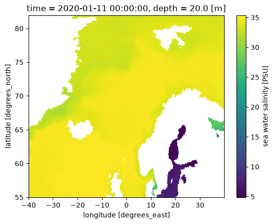
Run the two regridding steps separately#
regrid is just regrid_horizontal followed by regrid_vertical, and each is useful on its own.
To change only the vertical — put HYCOM’s hybrid layers onto fixed depth levels while keeping the native curvilinear horizontal grid — call regrid_vertical by itself. It needs no grid=, only thknss:
# Vertical only: hybrid layers -> z-levels; native curvilinear lon/lat (y, x) kept.
ds_v = xhycom.regrid_vertical(ds, depth=glorys["depth"].values)
ds_v
<xarray.Dataset> Size: 1TB
Dimensions:     (y: 380, x: 400, time: 366, ki: 51, depth: 50)
Coordinates:
    lon         (y, x) float64 1MB dask.array<chunksize=(380, 400), meta=np.ndarray>
    lat         (y, x) float64 1MB dask.array<chunksize=(380, 400), meta=np.ndarray>
    lon_u       (y, x) float64 1MB dask.array<chunksize=(380, 400), meta=np.ndarray>
    lat_u       (y, x) float64 1MB dask.array<chunksize=(380, 400), meta=np.ndarray>
    lon_v       (y, x) float64 1MB dask.array<chunksize=(380, 400), meta=np.ndarray>
    lat_v       (y, x) float64 1MB dask.array<chunksize=(380, 400), meta=np.ndarray>
  * time        (time) object 3kB 2020-01-01 00:00:00 ... 2020-12-31 00:00:00
  * ki          (ki) int64 408B 0 1 2 3 4 5 6 7 8 ... 42 43 44 45 46 47 48 49 50
  * depth       (depth) float64 400B 0.494 1.541 2.646 ... 5.275e+03 5.728e+03
Dimensions without coordinates: y, x
Data variables: (12/82)
    montg1      (time, y, x) float64 445MB dask.array<chunksize=(1, 380, 400), meta=np.ndarray>
    srfhgt      (time, y, x) float64 445MB dask.array<chunksize=(1, 380, 400), meta=np.ndarray>
    oneta       (time, y, x) float64 445MB dask.array<chunksize=(1, 380, 400), meta=np.ndarray>
    surflx      (time, y, x) float64 445MB dask.array<chunksize=(1, 380, 400), meta=np.ndarray>
    wtrflx      (time, y, x) float64 445MB dask.array<chunksize=(1, 380, 400), meta=np.ndarray>
    salflx      (time, y, x) float64 445MB dask.array<chunksize=(1, 380, 400), meta=np.ndarray>
    ...          ...
    ECO_c2ch_2  (time, y, x, depth) float64 22GB dask.array<chunksize=(1, 380, 400, 50), meta=np.ndarray>
    ECO_c2ch_3  (time, y, x, depth) float64 22GB dask.array<chunksize=(1, 380, 400, 50), meta=np.ndarray>
    light_sw    (time, y, x, depth) float64 22GB dask.array<chunksize=(1, 380, 400, 50), meta=np.ndarray>
    attenuat    (time, y, x, depth) float64 22GB dask.array<chunksize=(1, 380, 400, 50), meta=np.ndarray>
    total_ch    (time, y, x, depth) float64 22GB dask.array<chunksize=(1, 380, 400, 50), meta=np.ndarray>
    total_ca    (time, y, x, depth) float64 22GB dask.array<chunksize=(1, 380, 400, 50), meta=np.ndarray>
Attributes:
    iversn:        23
    iexpt:         28
    yrflag:        3
archive_type: mean- y: 380
- x: 400
- time: 366
- ki: 51
- depth: 50
- lon(y, x)float64dask.array<chunksize=(380, 400), meta=np.ndarray>
- long_name :
- longitude (T-point)
- units :
- degrees_east
- standard_name :
- longitude
Array Chunk Bytes 1.16 MiB 1.16 MiB Shape (380, 400) (380, 400) Dask graph 1 chunks in 1 graph layer Data type float64 numpy.ndarray - lat(y, x)float64dask.array<chunksize=(380, 400), meta=np.ndarray>
- long_name :
- latitude (T-point)
- units :
- degrees_north
- standard_name :
- latitude
Array Chunk Bytes 1.16 MiB 1.16 MiB Shape (380, 400) (380, 400) Dask graph 1 chunks in 1 graph layer Data type float64 numpy.ndarray - lon_u(y, x)float64dask.array<chunksize=(380, 400), meta=np.ndarray>
- long_name :
- longitude (U-point)
- units :
- degrees_east
Array Chunk Bytes 1.16 MiB 1.16 MiB Shape (380, 400) (380, 400) Dask graph 1 chunks in 1 graph layer Data type float64 numpy.ndarray - lat_u(y, x)float64dask.array<chunksize=(380, 400), meta=np.ndarray>
- long_name :
- latitude (U-point)
- units :
- degrees_north
Array Chunk Bytes 1.16 MiB 1.16 MiB Shape (380, 400) (380, 400) Dask graph 1 chunks in 1 graph layer Data type float64 numpy.ndarray - lon_v(y, x)float64dask.array<chunksize=(380, 400), meta=np.ndarray>
- long_name :
- longitude (V-point)
- units :
- degrees_east
Array Chunk Bytes 1.16 MiB 1.16 MiB Shape (380, 400) (380, 400) Dask graph 1 chunks in 1 graph layer Data type float64 numpy.ndarray - lat_v(y, x)float64dask.array<chunksize=(380, 400), meta=np.ndarray>
- long_name :
- latitude (V-point)
- units :
- degrees_north
Array Chunk Bytes 1.16 MiB 1.16 MiB Shape (380, 400) (380, 400) Dask graph 1 chunks in 1 graph layer Data type float64 numpy.ndarray - time(time)object2020-01-01 00:00:00 ... 2020-12-...
- long_name :
- time
- axis :
- T
array([cftime.DatetimeGregorian(2020, 1, 1, 0, 0, 0, 0, has_year_zero=False), cftime.DatetimeGregorian(2020, 1, 2, 0, 0, 0, 0, has_year_zero=False), cftime.DatetimeGregorian(2020, 1, 3, 0, 0, 0, 0, has_year_zero=False), ..., cftime.DatetimeGregorian(2020, 12, 29, 0, 0, 0, 0, has_year_zero=False), cftime.DatetimeGregorian(2020, 12, 30, 0, 0, 0, 0, has_year_zero=False), cftime.DatetimeGregorian(2020, 12, 31, 0, 0, 0, 0, has_year_zero=False)], shape=(366,), dtype=object) - ki(ki)int640 1 2 3 4 5 6 ... 45 46 47 48 49 50
- long_name :
- layer interface index
- units :
- 1
- axis :
- Z
array([ 0, 1, 2, 3, 4, 5, 6, 7, 8, 9, 10, 11, 12, 13, 14, 15, 16, 17, 18, 19, 20, 21, 22, 23, 24, 25, 26, 27, 28, 29, 30, 31, 32, 33, 34, 35, 36, 37, 38, 39, 40, 41, 42, 43, 44, 45, 46, 47, 48, 49, 50]) - depth(depth)float640.494 1.541 ... 5.275e+03 5.728e+03
- long_name :
- depth
- units :
- m
- positive :
- down
- axis :
- Z
array([4.940250e-01, 1.541375e+00, 2.645669e+00, 3.819495e+00, 5.078224e+00,
       6.440614e+00, 7.929560e+00, 9.572997e+00, 1.140500e+01, 1.346714e+01,
       1.581007e+01, 1.849556e+01, 2.159882e+01, 2.521141e+01, 2.944473e+01,
       3.443415e+01, 4.034405e+01, 4.737369e+01, 5.576429e+01, 6.580727e+01,
       7.785385e+01, 9.232607e+01, 1.097293e+02, 1.306660e+02, 1.558507e+02,
       1.861256e+02, 2.224752e+02, 2.660403e+02, 3.181274e+02, 3.802130e+02,
       4.539377e+02, 5.410889e+02, 6.435668e+02, 7.633331e+02, 9.023393e+02,
       1.062440e+03, 1.245291e+03, 1.452251e+03, 1.684284e+03, 1.941893e+03,
       2.225078e+03, 2.533336e+03, 2.865703e+03, 3.220820e+03, 3.597032e+03,
       3.992484e+03, 4.405224e+03, 4.833291e+03, 5.274784e+03, 5.727917e+03])
- montg1(time, y, x)float64dask.array<chunksize=(1, 380, 400), meta=np.ndarray>
- long_name :
- Montgomery potential
- units :
- m2 s-2
Array Chunk Bytes 424.44 MiB 1.16 MiB Shape (366, 380, 400) (1, 380, 400) Dask graph 366 chunks in 733 graph layers Data type float64 numpy.ndarray - srfhgt(time, y, x)float64dask.array<chunksize=(1, 380, 400), meta=np.ndarray>
- long_name :
- sea surface height
- units :
- m
- comment :
- converted from Pa (factor 0.101978)
Array Chunk Bytes 424.44 MiB 1.16 MiB Shape (366, 380, 400) (1, 380, 400) Dask graph 366 chunks in 734 graph layers Data type float64 numpy.ndarray - oneta(time, y, x)float64dask.array<chunksize=(1, 380, 400), meta=np.ndarray>
- long_name :
- free surface elevation
- units :
- m
Array Chunk Bytes 424.44 MiB 1.16 MiB Shape (366, 380, 400) (1, 380, 400) Dask graph 366 chunks in 733 graph layers Data type float64 numpy.ndarray - surflx(time, y, x)float64dask.array<chunksize=(1, 380, 400), meta=np.ndarray>
- long_name :
- net surface heat flux
- units :
- W m-2
Array Chunk Bytes 424.44 MiB 1.16 MiB Shape (366, 380, 400) (1, 380, 400) Dask graph 366 chunks in 733 graph layers Data type float64 numpy.ndarray - wtrflx(time, y, x)float64dask.array<chunksize=(1, 380, 400), meta=np.ndarray>
- long_name :
- net surface freshwater flux
- units :
- m s-1
Array Chunk Bytes 424.44 MiB 1.16 MiB Shape (366, 380, 400) (1, 380, 400) Dask graph 366 chunks in 733 graph layers Data type float64 numpy.ndarray - salflx(time, y, x)float64dask.array<chunksize=(1, 380, 400), meta=np.ndarray>
- long_name :
- surface salt flux
- units :
- PSU m s-1
Array Chunk Bytes 424.44 MiB 1.16 MiB Shape (366, 380, 400) (1, 380, 400) Dask graph 366 chunks in 733 graph layers Data type float64 numpy.ndarray - bl_dpth(time, y, x)float64dask.array<chunksize=(1, 380, 400), meta=np.ndarray>
- long_name :
- boundary layer depth
- units :
- m
- comment :
- converted from Pa (factor 0.000101978)
Array Chunk Bytes 424.44 MiB 1.16 MiB Shape (366, 380, 400) (1, 380, 400) Dask graph 366 chunks in 734 graph layers Data type float64 numpy.ndarray - mix_dpth(time, y, x)float64dask.array<chunksize=(1, 380, 400), meta=np.ndarray>
- long_name :
- mixed layer depth
- units :
- m
- comment :
- converted from Pa (factor 0.000101978)
Array Chunk Bytes 424.44 MiB 1.16 MiB Shape (366, 380, 400) (1, 380, 400) Dask graph 366 chunks in 734 graph layers Data type float64 numpy.ndarray - tmix(time, y, x)float64dask.array<chunksize=(1, 380, 400), meta=np.ndarray>
- long_name :
- mixed layer temperature
- units :
- degC
Array Chunk Bytes 424.44 MiB 1.16 MiB Shape (366, 380, 400) (1, 380, 400) Dask graph 366 chunks in 733 graph layers Data type float64 numpy.ndarray - smix(time, y, x)float64dask.array<chunksize=(1, 380, 400), meta=np.ndarray>
- long_name :
- mixed layer salinity
- units :
- PSU
Array Chunk Bytes 424.44 MiB 1.16 MiB Shape (366, 380, 400) (1, 380, 400) Dask graph 366 chunks in 733 graph layers Data type float64 numpy.ndarray - thmix(time, y, x)float64dask.array<chunksize=(1, 380, 400), meta=np.ndarray>
- long_name :
- mixed layer thickness
- units :
- m
- comment :
- converted from Pa (factor 0.000101978)
Array Chunk Bytes 424.44 MiB 1.16 MiB Shape (366, 380, 400) (1, 380, 400) Dask graph 366 chunks in 734 graph layers Data type float64 numpy.ndarray - umix(time, y, x)float64dask.array<chunksize=(1, 380, 400), meta=np.ndarray>
- long_name :
- mixed layer x velocity
- units :
- m s-1
Array Chunk Bytes 424.44 MiB 1.16 MiB Shape (366, 380, 400) (1, 380, 400) Dask graph 366 chunks in 733 graph layers Data type float64 numpy.ndarray - vmix(time, y, x)float64dask.array<chunksize=(1, 380, 400), meta=np.ndarray>
- long_name :
- mixed layer y velocity
- units :
- m s-1
Array Chunk Bytes 424.44 MiB 1.16 MiB Shape (366, 380, 400) (1, 380, 400) Dask graph 366 chunks in 733 graph layers Data type float64 numpy.ndarray - kemix(time, y, x)float64dask.array<chunksize=(1, 380, 400), meta=np.ndarray>
- long_name :
- mixed layer kinetic energy
- units :
- m2 s-2
Array Chunk Bytes 424.44 MiB 1.16 MiB Shape (366, 380, 400) (1, 380, 400) Dask graph 366 chunks in 733 graph layers Data type float64 numpy.ndarray - covice(time, y, x)float64dask.array<chunksize=(1, 380, 400), meta=np.ndarray>
- long_name :
- sea ice coverage fraction
- units :
- 1
Array Chunk Bytes 424.44 MiB 1.16 MiB Shape (366, 380, 400) (1, 380, 400) Dask graph 366 chunks in 733 graph layers Data type float64 numpy.ndarray - thkice(time, y, x)float64dask.array<chunksize=(1, 380, 400), meta=np.ndarray>
- long_name :
- sea ice thickness
- units :
- m
Array Chunk Bytes 424.44 MiB 1.16 MiB Shape (366, 380, 400) (1, 380, 400) Dask graph 366 chunks in 733 graph layers Data type float64 numpy.ndarray - temice(time, y, x)float64dask.array<chunksize=(1, 380, 400), meta=np.ndarray>
- long_name :
- sea ice surface temperature
- units :
- degC
Array Chunk Bytes 424.44 MiB 1.16 MiB Shape (366, 380, 400) (1, 380, 400) Dask graph 366 chunks in 733 graph layers Data type float64 numpy.ndarray - u_btrop(time, y, x)float64dask.array<chunksize=(1, 380, 400), meta=np.ndarray>
- long_name :
- barotropic x velocity
- units :
- m s-1
Array Chunk Bytes 424.44 MiB 1.16 MiB Shape (366, 380, 400) (1, 380, 400) Dask graph 366 chunks in 733 graph layers Data type float64 numpy.ndarray - v_btrop(time, y, x)float64dask.array<chunksize=(1, 380, 400), meta=np.ndarray>
- long_name :
- barotropic y velocity
- units :
- m s-1
Array Chunk Bytes 424.44 MiB 1.16 MiB Shape (366, 380, 400) (1, 380, 400) Dask graph 366 chunks in 733 graph layers Data type float64 numpy.ndarray - kebtrop(time, y, x)float64dask.array<chunksize=(1, 380, 400), meta=np.ndarray>
- long_name :
- barotropic kinetic energy
- units :
- m2 s-2
Array Chunk Bytes 424.44 MiB 1.16 MiB Shape (366, 380, 400) (1, 380, 400) Dask graph 366 chunks in 733 graph layers Data type float64 numpy.ndarray - light_pa(time, ki, y, x)float64dask.array<chunksize=(1, 51, 380, 400), meta=np.ndarray>
- long_name :
- PAR irradiance
- units :
- W m-2
Array Chunk Bytes 21.14 GiB 59.14 MiB Shape (366, 51, 380, 400) (1, 51, 380, 400) Dask graph 366 chunks in 733 graph layers Data type float64 numpy.ndarray - ECO_sed4(time, y, x)float64dask.array<chunksize=(1, 380, 400), meta=np.ndarray>
- long_name :
- sediment pool 4
- units :
- mmol m-2
Array Chunk Bytes 424.44 MiB 1.16 MiB Shape (366, 380, 400) (1, 380, 400) Dask graph 366 chunks in 733 graph layers Data type float64 numpy.ndarray - ECO_sed1(time, y, x)float64dask.array<chunksize=(1, 380, 400), meta=np.ndarray>
- long_name :
- sediment pool 1
- units :
- mmol m-2
Array Chunk Bytes 424.44 MiB 1.16 MiB Shape (366, 380, 400) (1, 380, 400) Dask graph 366 chunks in 733 graph layers Data type float64 numpy.ndarray - ECO_sed2(time, y, x)float64dask.array<chunksize=(1, 380, 400), meta=np.ndarray>
- long_name :
- sediment pool 2
- units :
- mmol m-2
Array Chunk Bytes 424.44 MiB 1.16 MiB Shape (366, 380, 400) (1, 380, 400) Dask graph 366 chunks in 733 graph layers Data type float64 numpy.ndarray - ECO_sed3(time, y, x)float64dask.array<chunksize=(1, 380, 400), meta=np.ndarray>
- long_name :
- sediment pool 3
- units :
- mmol m-2
Array Chunk Bytes 424.44 MiB 1.16 MiB Shape (366, 380, 400) (1, 380, 400) Dask graph 366 chunks in 733 graph layers Data type float64 numpy.ndarray - CO2_fair(time, y, x)float64dask.array<chunksize=(1, 380, 400), meta=np.ndarray>
- long_name :
- air-sea CO2 flux
- units :
- mmol C m-2 d-1
Array Chunk Bytes 424.44 MiB 1.16 MiB Shape (366, 380, 400) (1, 380, 400) Dask graph 366 chunks in 733 graph layers Data type float64 numpy.ndarray - CO2_wind(time, y, x)float64dask.array<chunksize=(1, 380, 400), meta=np.ndarray>
- long_name :
- wind speed for gas exchange
- units :
- m s-1
Array Chunk Bytes 424.44 MiB 1.16 MiB Shape (366, 380, 400) (1, 380, 400) Dask graph 366 chunks in 733 graph layers Data type float64 numpy.ndarray - ECO_bots(time, y, x)float64dask.array<chunksize=(1, 380, 400), meta=np.ndarray>
- long_name :
- bottom sediment flux
- units :
- 1
Array Chunk Bytes 424.44 MiB 1.16 MiB Shape (366, 380, 400) (1, 380, 400) Dask graph 366 chunks in 733 graph layers Data type float64 numpy.ndarray - surface__1(time, y, x)float64dask.array<chunksize=(1, 380, 400), meta=np.ndarray>
Array Chunk Bytes 424.44 MiB 1.16 MiB Shape (366, 380, 400) (1, 380, 400) Dask graph 366 chunks in 733 graph layers Data type float64 numpy.ndarray - surface__2(time, y, x)float64dask.array<chunksize=(1, 380, 400), meta=np.ndarray>
Array Chunk Bytes 424.44 MiB 1.16 MiB Shape (366, 380, 400) (1, 380, 400) Dask graph 366 chunks in 733 graph layers Data type float64 numpy.ndarray - si_u(time, y, x)float64dask.array<chunksize=(1, 380, 400), meta=np.ndarray>
- long_name :
- sea ice x velocity
- units :
- m s-1
Array Chunk Bytes 424.44 MiB 1.16 MiB Shape (366, 380, 400) (1, 380, 400) Dask graph 366 chunks in 733 graph layers Data type float64 numpy.ndarray - si_v(time, y, x)float64dask.array<chunksize=(1, 380, 400), meta=np.ndarray>
- long_name :
- sea ice y velocity
- units :
- m s-1
Array Chunk Bytes 424.44 MiB 1.16 MiB Shape (366, 380, 400) (1, 380, 400) Dask graph 366 chunks in 733 graph layers Data type float64 numpy.ndarray - u-vel.(time, y, x, depth)float64dask.array<chunksize=(1, 380, 400, 50), meta=np.ndarray>
- long_name :
- sea water x velocity
- units :
- m s-1
- hycom_velocity :
- total
- comment :
- total current (baroclinic + barotropic); the barotropic part was summed in when the archm time mean was formed
Array Chunk Bytes 20.72 GiB 57.98 MiB Shape (366, 380, 400, 50) (1, 380, 400, 50) Dask graph 366 chunks in 1489 graph layers Data type float64 numpy.ndarray - v-vel.(time, y, x, depth)float64dask.array<chunksize=(1, 380, 400, 50), meta=np.ndarray>
- long_name :
- sea water y velocity
- units :
- m s-1
- hycom_velocity :
- total
- comment :
- total current (baroclinic + barotropic); the barotropic part was summed in when the archm time mean was formed
Array Chunk Bytes 20.72 GiB 57.98 MiB Shape (366, 380, 400, 50) (1, 380, 400, 50) Dask graph 366 chunks in 1489 graph layers Data type float64 numpy.ndarray - k.e.(time, y, x, depth)float64dask.array<chunksize=(1, 380, 400, 50), meta=np.ndarray>
- long_name :
- kinetic energy
- units :
- m2 s-2
Array Chunk Bytes 20.72 GiB 57.98 MiB Shape (366, 380, 400, 50) (1, 380, 400, 50) Dask graph 366 chunks in 1489 graph layers Data type float64 numpy.ndarray - temp(time, y, x, depth)float64dask.array<chunksize=(1, 380, 400, 50), meta=np.ndarray>
- long_name :
- sea water potential temperature
- units :
- degC
Array Chunk Bytes 20.72 GiB 57.98 MiB Shape (366, 380, 400, 50) (1, 380, 400, 50) Dask graph 366 chunks in 1489 graph layers Data type float64 numpy.ndarray - salin(time, y, x, depth)float64dask.array<chunksize=(1, 380, 400, 50), meta=np.ndarray>
- long_name :
- sea water salinity
- units :
- PSU
Array Chunk Bytes 20.72 GiB 57.98 MiB Shape (366, 380, 400, 50) (1, 380, 400, 50) Dask graph 366 chunks in 1489 graph layers Data type float64 numpy.ndarray - density(time, y, x, depth)float64dask.array<chunksize=(1, 380, 400, 50), meta=np.ndarray>
- long_name :
- sea water potential density (sigma-2)
- units :
- kg m-3
Array Chunk Bytes 20.72 GiB 57.98 MiB Shape (366, 380, 400, 50) (1, 380, 400, 50) Dask graph 366 chunks in 1489 graph layers Data type float64 numpy.ndarray - CO2_c(time, y, x, depth)float64dask.array<chunksize=(1, 380, 400, 50), meta=np.ndarray>
- long_name :
- dissolved inorganic carbon
- units :
- mmol C m-3
Array Chunk Bytes 20.72 GiB 57.98 MiB Shape (366, 380, 400, 50) (1, 380, 400, 50) Dask graph 366 chunks in 1489 graph layers Data type float64 numpy.ndarray - CO2_TA(time, y, x, depth)float64dask.array<chunksize=(1, 380, 400, 50), meta=np.ndarray>
- long_name :
- total alkalinity
- units :
- mmol eq m-3
Array Chunk Bytes 20.72 GiB 57.98 MiB Shape (366, 380, 400, 50) (1, 380, 400, 50) Dask graph 366 chunks in 1489 graph layers Data type float64 numpy.ndarray - ECO_no3(time, y, x, depth)float64dask.array<chunksize=(1, 380, 400, 50), meta=np.ndarray>
- long_name :
- nitrate
- units :
- mmol N m-3
Array Chunk Bytes 20.72 GiB 57.98 MiB Shape (366, 380, 400, 50) (1, 380, 400, 50) Dask graph 366 chunks in 1489 graph layers Data type float64 numpy.ndarray - ECO_nh4(time, y, x, depth)float64dask.array<chunksize=(1, 380, 400, 50), meta=np.ndarray>
- long_name :
- ammonium
- units :
- mmol N m-3
Array Chunk Bytes 20.72 GiB 57.98 MiB Shape (366, 380, 400, 50) (1, 380, 400, 50) Dask graph 366 chunks in 1489 graph layers Data type float64 numpy.ndarray - ECO_pho(time, y, x, depth)float64dask.array<chunksize=(1, 380, 400, 50), meta=np.ndarray>
- long_name :
- phosphate
- units :
- mmol P m-3
Array Chunk Bytes 20.72 GiB 57.98 MiB Shape (366, 380, 400, 50) (1, 380, 400, 50) Dask graph 366 chunks in 1489 graph layers Data type float64 numpy.ndarray - ECO_sil(time, y, x, depth)float64dask.array<chunksize=(1, 380, 400, 50), meta=np.ndarray>
- long_name :
- silicate
- units :
- mmol Si m-3
Array Chunk Bytes 20.72 GiB 57.98 MiB Shape (366, 380, 400, 50) (1, 380, 400, 50) Dask graph 366 chunks in 1489 graph layers Data type float64 numpy.ndarray - ECO_oxy(time, y, x, depth)float64dask.array<chunksize=(1, 380, 400, 50), meta=np.ndarray>
- long_name :
- dissolved oxygen
- units :
- mmol O m-3
Array Chunk Bytes 20.72 GiB 57.98 MiB Shape (366, 380, 400, 50) (1, 380, 400, 50) Dask graph 366 chunks in 1489 graph layers Data type float64 numpy.ndarray - ECO_fla(time, y, x, depth)float64dask.array<chunksize=(1, 380, 400, 50), meta=np.ndarray>
- long_name :
- flagellate carbon
- units :
- mmol C m-3
Array Chunk Bytes 20.72 GiB 57.98 MiB Shape (366, 380, 400, 50) (1, 380, 400, 50) Dask graph 366 chunks in 1489 graph layers Data type float64 numpy.ndarray - ECO_dia(time, y, x, depth)float64dask.array<chunksize=(1, 380, 400, 50), meta=np.ndarray>
- long_name :
- diatom carbon
- units :
- mmol C m-3
Array Chunk Bytes 20.72 GiB 57.98 MiB Shape (366, 380, 400, 50) (1, 380, 400, 50) Dask graph 366 chunks in 1489 graph layers Data type float64 numpy.ndarray - ECO_ccl(time, y, x, depth)float64dask.array<chunksize=(1, 380, 400, 50), meta=np.ndarray>
- long_name :
- coccolithophore carbon
- units :
- mmol C m-3
Array Chunk Bytes 20.72 GiB 57.98 MiB Shape (366, 380, 400, 50) (1, 380, 400, 50) Dask graph 366 chunks in 1489 graph layers Data type float64 numpy.ndarray - ECO_cclc(time, y, x, depth)float64dask.array<chunksize=(1, 380, 400, 50), meta=np.ndarray>
- long_name :
- coccolithophore calcite carbon
- units :
- mmol C m-3
Array Chunk Bytes 20.72 GiB 57.98 MiB Shape (366, 380, 400, 50) (1, 380, 400, 50) Dask graph 366 chunks in 1489 graph layers Data type float64 numpy.ndarray - ECO_caco(time, y, x, depth)float64dask.array<chunksize=(1, 380, 400, 50), meta=np.ndarray>
- long_name :
- particulate inorganic carbon (calcite)
- units :
- mmol C m-3
Array Chunk Bytes 20.72 GiB 57.98 MiB Shape (366, 380, 400, 50) (1, 380, 400, 50) Dask graph 366 chunks in 1489 graph layers Data type float64 numpy.ndarray - ECO_diac(time, y, x, depth)float64dask.array<chunksize=(1, 380, 400, 50), meta=np.ndarray>
- long_name :
- diatom calcite carbon
- units :
- mmol C m-3
Array Chunk Bytes 20.72 GiB 57.98 MiB Shape (366, 380, 400, 50) (1, 380, 400, 50) Dask graph 366 chunks in 1489 graph layers Data type float64 numpy.ndarray - ECO_flac(time, y, x, depth)float64dask.array<chunksize=(1, 380, 400, 50), meta=np.ndarray>
- long_name :
- flagellate calcite carbon
- units :
- mmol C m-3
Array Chunk Bytes 20.72 GiB 57.98 MiB Shape (366, 380, 400, 50) (1, 380, 400, 50) Dask graph 366 chunks in 1489 graph layers Data type float64 numpy.ndarray - ECO_micr(time, y, x, depth)float64dask.array<chunksize=(1, 380, 400, 50), meta=np.ndarray>
- long_name :
- microzooplankton carbon
- units :
- mmol C m-3
Array Chunk Bytes 20.72 GiB 57.98 MiB Shape (366, 380, 400, 50) (1, 380, 400, 50) Dask graph 366 chunks in 1489 graph layers Data type float64 numpy.ndarray - ECO_meso(time, y, x, depth)float64dask.array<chunksize=(1, 380, 400, 50), meta=np.ndarray>
- long_name :
- mesozooplankton carbon
- units :
- mmol C m-3
Array Chunk Bytes 20.72 GiB 57.98 MiB Shape (366, 380, 400, 50) (1, 380, 400, 50) Dask graph 366 chunks in 1489 graph layers Data type float64 numpy.ndarray - ECO_det(time, y, x, depth)float64dask.array<chunksize=(1, 380, 400, 50), meta=np.ndarray>
- long_name :
- detritus carbon
- units :
- mmol C m-3
Array Chunk Bytes 20.72 GiB 57.98 MiB Shape (366, 380, 400, 50) (1, 380, 400, 50) Dask graph 366 chunks in 1489 graph layers Data type float64 numpy.ndarray - ECO_opa(time, y, x, depth)float64dask.array<chunksize=(1, 380, 400, 50), meta=np.ndarray>
- long_name :
- opal (biogenic silica)
- units :
- mmol Si m-3
Array Chunk Bytes 20.72 GiB 57.98 MiB Shape (366, 380, 400, 50) (1, 380, 400, 50) Dask graph 366 chunks in 1489 graph layers Data type float64 numpy.ndarray - ECO_dom(time, y, x, depth)float64dask.array<chunksize=(1, 380, 400, 50), meta=np.ndarray>
- long_name :
- dissolved organic matter carbon
- units :
- mmol C m-3
Array Chunk Bytes 20.72 GiB 57.98 MiB Shape (366, 380, 400, 50) (1, 380, 400, 50) Dask graph 366 chunks in 1489 graph layers Data type float64 numpy.ndarray - ECO_dsnk(time, y, x, depth)float64dask.array<chunksize=(1, 380, 400, 50), meta=np.ndarray>
- long_name :
- detritus sinking flux
- units :
- mmol C m-2 s-1
Array Chunk Bytes 20.72 GiB 57.98 MiB Shape (366, 380, 400, 50) (1, 380, 400, 50) Dask graph 366 chunks in 1489 graph layers Data type float64 numpy.ndarray - CO2_pH(time, y, x, depth)float64dask.array<chunksize=(1, 380, 400, 50), meta=np.ndarray>
- long_name :
- seawater pH
- units :
- 1
Array Chunk Bytes 20.72 GiB 57.98 MiB Shape (366, 380, 400, 50) (1, 380, 400, 50) Dask graph 366 chunks in 1489 graph layers Data type float64 numpy.ndarray - CO2_pCO2(time, y, x, depth)float64dask.array<chunksize=(1, 380, 400, 50), meta=np.ndarray>
- long_name :
- partial pressure of CO2
- units :
- uatm
Array Chunk Bytes 20.72 GiB 57.98 MiB Shape (366, 380, 400, 50) (1, 380, 400, 50) Dask graph 366 chunks in 1489 graph layers Data type float64 numpy.ndarray - CO2_Carb_1(time, y, x, depth)float64dask.array<chunksize=(1, 380, 400, 50), meta=np.ndarray>
- long_name :
- carbonate concentration
- units :
- mmol C m-3
Array Chunk Bytes 20.72 GiB 57.98 MiB Shape (366, 380, 400, 50) (1, 380, 400, 50) Dask graph 366 chunks in 1489 graph layers Data type float64 numpy.ndarray - CO2_BiCa(time, y, x, depth)float64dask.array<chunksize=(1, 380, 400, 50), meta=np.ndarray>
- long_name :
- bicarbonate concentration
- units :
- mmol C m-3
Array Chunk Bytes 20.72 GiB 57.98 MiB Shape (366, 380, 400, 50) (1, 380, 400, 50) Dask graph 366 chunks in 1489 graph layers Data type float64 numpy.ndarray - CO2_Carb_2(time, y, x, depth)float64dask.array<chunksize=(1, 380, 400, 50), meta=np.ndarray>
- long_name :
- carbonate concentration
- units :
- mmol C m-3
Array Chunk Bytes 20.72 GiB 57.98 MiB Shape (366, 380, 400, 50) (1, 380, 400, 50) Dask graph 366 chunks in 1489 graph layers Data type float64 numpy.ndarray - CO2_Om_c(time, y, x, depth)float64dask.array<chunksize=(1, 380, 400, 50), meta=np.ndarray>
- long_name :
- calcite saturation state (Omega)
- units :
- 1
Array Chunk Bytes 20.72 GiB 57.98 MiB Shape (366, 380, 400, 50) (1, 380, 400, 50) Dask graph 366 chunks in 1489 graph layers Data type float64 numpy.ndarray - CO2_Om_a(time, y, x, depth)float64dask.array<chunksize=(1, 380, 400, 50), meta=np.ndarray>
- long_name :
- aragonite saturation state (Omega)
- units :
- 1
Array Chunk Bytes 20.72 GiB 57.98 MiB Shape (366, 380, 400, 50) (1, 380, 400, 50) Dask graph 366 chunks in 1489 graph layers Data type float64 numpy.ndarray - ECO_prim(time, y, x, depth)float64dask.array<chunksize=(1, 380, 400, 50), meta=np.ndarray>
- long_name :
- primary production
- units :
- mmol C m-3 s-1
Array Chunk Bytes 20.72 GiB 57.98 MiB Shape (366, 380, 400, 50) (1, 380, 400, 50) Dask graph 366 chunks in 1489 graph layers Data type float64 numpy.ndarray - ECO_secp(time, y, x, depth)float64dask.array<chunksize=(1, 380, 400, 50), meta=np.ndarray>
- long_name :
- secondary production
- units :
- mmol C m-3 s-1
Array Chunk Bytes 20.72 GiB 57.98 MiB Shape (366, 380, 400, 50) (1, 380, 400, 50) Dask graph 366 chunks in 1489 graph layers Data type float64 numpy.ndarray - ECO_netp(time, y, x, depth)float64dask.array<chunksize=(1, 380, 400, 50), meta=np.ndarray>
- long_name :
- net primary production
- units :
- mmol C m-3 s-1
Array Chunk Bytes 20.72 GiB 57.98 MiB Shape (366, 380, 400, 50) (1, 380, 400, 50) Dask graph 366 chunks in 1489 graph layers Data type float64 numpy.ndarray - ECO_parm(time, y, x, depth)float64dask.array<chunksize=(1, 380, 400, 50), meta=np.ndarray>
- long_name :
- BGC parameter field
- units :
- 1
Array Chunk Bytes 20.72 GiB 57.98 MiB Shape (366, 380, 400, 50) (1, 380, 400, 50) Dask graph 366 chunks in 1489 graph layers Data type float64 numpy.ndarray - ECO_Nlim(time, y, x, depth)float64dask.array<chunksize=(1, 380, 400, 50), meta=np.ndarray>
- long_name :
- nitrogen limitation factor
- units :
- 1
Array Chunk Bytes 20.72 GiB 57.98 MiB Shape (366, 380, 400, 50) (1, 380, 400, 50) Dask graph 366 chunks in 1489 graph layers Data type float64 numpy.ndarray - ECO_Plim(time, y, x, depth)float64dask.array<chunksize=(1, 380, 400, 50), meta=np.ndarray>
- long_name :
- phosphorus limitation factor
- units :
- 1
Array Chunk Bytes 20.72 GiB 57.98 MiB Shape (366, 380, 400, 50) (1, 380, 400, 50) Dask graph 366 chunks in 1489 graph layers Data type float64 numpy.ndarray - ECO_Slim(time, y, x, depth)float64dask.array<chunksize=(1, 380, 400, 50), meta=np.ndarray>
- long_name :
- silicate limitation factor
- units :
- 1
Array Chunk Bytes 20.72 GiB 57.98 MiB Shape (366, 380, 400, 50) (1, 380, 400, 50) Dask graph 366 chunks in 1489 graph layers Data type float64 numpy.ndarray - ECO_Llim(time, y, x, depth)float64dask.array<chunksize=(1, 380, 400, 50), meta=np.ndarray>
- long_name :
- light limitation factor
- units :
- 1
Array Chunk Bytes 20.72 GiB 57.98 MiB Shape (366, 380, 400, 50) (1, 380, 400, 50) Dask graph 366 chunks in 1489 graph layers Data type float64 numpy.ndarray - ECO_deni(time, y, x, depth)float64dask.array<chunksize=(1, 380, 400, 50), meta=np.ndarray>
- long_name :
- denitrification
- units :
- mmol N m-3 s-1
Array Chunk Bytes 20.72 GiB 57.98 MiB Shape (366, 380, 400, 50) (1, 380, 400, 50) Dask graph 366 chunks in 1489 graph layers Data type float64 numpy.ndarray - ECO_snks(time, y, x, depth)float64dask.array<chunksize=(1, 380, 400, 50), meta=np.ndarray>
- long_name :
- sinking rate
- units :
- m d-1
Array Chunk Bytes 20.72 GiB 57.98 MiB Shape (366, 380, 400, 50) (1, 380, 400, 50) Dask graph 366 chunks in 1489 graph layers Data type float64 numpy.ndarray - ECO_c2ch_1(time, y, x, depth)float64dask.array<chunksize=(1, 380, 400, 50), meta=np.ndarray>
- long_name :
- carbon to chlorophyll ratio
- units :
- g C g-1 Chl
Array Chunk Bytes 20.72 GiB 57.98 MiB Shape (366, 380, 400, 50) (1, 380, 400, 50) Dask graph 366 chunks in 1489 graph layers Data type float64 numpy.ndarray - ECO_c2ch_2(time, y, x, depth)float64dask.array<chunksize=(1, 380, 400, 50), meta=np.ndarray>
- long_name :
- carbon to chlorophyll ratio
- units :
- g C g-1 Chl
Array Chunk Bytes 20.72 GiB 57.98 MiB Shape (366, 380, 400, 50) (1, 380, 400, 50) Dask graph 366 chunks in 1489 graph layers Data type float64 numpy.ndarray - ECO_c2ch_3(time, y, x, depth)float64dask.array<chunksize=(1, 380, 400, 50), meta=np.ndarray>
- long_name :
- carbon to chlorophyll ratio
- units :
- g C g-1 Chl
Array Chunk Bytes 20.72 GiB 57.98 MiB Shape (366, 380, 400, 50) (1, 380, 400, 50) Dask graph 366 chunks in 1489 graph layers Data type float64 numpy.ndarray - light_sw(time, y, x, depth)float64dask.array<chunksize=(1, 380, 400, 50), meta=np.ndarray>
- long_name :
- shortwave irradiance in water
- units :
- W m-2
Array Chunk Bytes 20.72 GiB 57.98 MiB Shape (366, 380, 400, 50) (1, 380, 400, 50) Dask graph 366 chunks in 1489 graph layers Data type float64 numpy.ndarray - attenuat(time, y, x, depth)float64dask.array<chunksize=(1, 380, 400, 50), meta=np.ndarray>
- long_name :
- light attenuation coefficient
- units :
- m-1
Array Chunk Bytes 20.72 GiB 57.98 MiB Shape (366, 380, 400, 50) (1, 380, 400, 50) Dask graph 366 chunks in 1489 graph layers Data type float64 numpy.ndarray - total_ch(time, y, x, depth)float64dask.array<chunksize=(1, 380, 400, 50), meta=np.ndarray>
- long_name :
- total chlorophyll
- units :
- mg Chl m-3
Array Chunk Bytes 20.72 GiB 57.98 MiB Shape (366, 380, 400, 50) (1, 380, 400, 50) Dask graph 366 chunks in 1489 graph layers Data type float64 numpy.ndarray - total_ca(time, y, x, depth)float64dask.array<chunksize=(1, 380, 400, 50), meta=np.ndarray>
- long_name :
- total carbon
- units :
- mmol C m-3
Array Chunk Bytes 20.72 GiB 57.98 MiB Shape (366, 380, 400, 50) (1, 380, 400, 50) Dask graph 366 chunks in 1489 graph layers Data type float64 numpy.ndarray
- iversn :
- 23
- iexpt :
- 28
- yrflag :
- 3
- archive_type :
- mean
ds_v.salin.isel(time=0).sel(depth=50, method="nearest").plot()
<matplotlib.collections.QuadMesh at 0x14d828bf0a50>
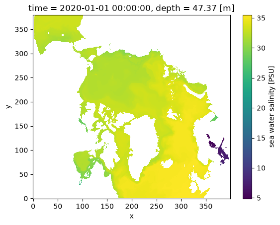
Or change only the horizontal — map the curvilinear grid to regular lon/lat while keeping the hybrid layers (k). This step needs grid= (it supplies pang to rotate velocities and qlon/qlat for conservative cell corners):
ds_h = xhycom.regrid_horizontal(ds, target=glorys, grid=grid)   # curvilinear -> regular lon/lat
ds_h
<xarray.Dataset> Size: 21TB
Dimensions:     (time: 366, lat: 624, lon: 4320, k: 50, ki: 51, y_b: 381,
                 x_b: 401)
Coordinates:
  * time        (time) object 3kB 2020-01-01 00:00:00 ... 2020-12-31 00:00:00
  * lat         (lat) float32 2kB 38.08 38.17 38.25 38.33 ... 89.83 89.92 90.0
  * lon         (lon) float32 17kB -180.0 -179.9 -179.8 ... 179.8 179.8 179.9
  * k           (k) int64 400B 1 2 3 4 5 6 7 8 9 ... 42 43 44 45 46 47 48 49 50
    dens        (k) float64 400B dask.array<chunksize=(50,), meta=np.ndarray>
  * ki          (ki) int64 408B 0 1 2 3 4 5 6 7 8 ... 42 43 44 45 46 47 48 49 50
    lon_b       (y_b, x_b) float64 1MB -94.76 -94.6 -94.43 ... 99.11 98.97 98.84
    lat_b       (y_b, x_b) float64 1MB 38.94 39.04 39.14 ... 56.3 56.21 56.12
Dimensions without coordinates: y_b, x_b
Data variables: (12/83)
    montg1      (time, lat, lon) float64 8GB dask.array<chunksize=(1, 624, 4320), meta=np.ndarray>
    srfhgt      (time, lat, lon) float64 8GB dask.array<chunksize=(1, 624, 4320), meta=np.ndarray>
    oneta       (time, lat, lon) float64 8GB dask.array<chunksize=(1, 624, 4320), meta=np.ndarray>
    surflx      (time, lat, lon) float64 8GB dask.array<chunksize=(1, 624, 4320), meta=np.ndarray>
    wtrflx      (time, lat, lon) float64 8GB dask.array<chunksize=(1, 624, 4320), meta=np.ndarray>
    salflx      (time, lat, lon) float64 8GB dask.array<chunksize=(1, 624, 4320), meta=np.ndarray>
    ...          ...
    u_btrop     (time, lat, lon) float64 8GB dask.array<chunksize=(1, 624, 4320), meta=np.ndarray>
    v_btrop     (time, lat, lon) float64 8GB dask.array<chunksize=(1, 624, 4320), meta=np.ndarray>
    umix        (time, lat, lon) float64 8GB dask.array<chunksize=(1, 624, 4320), meta=np.ndarray>
    vmix        (time, lat, lon) float64 8GB dask.array<chunksize=(1, 624, 4320), meta=np.ndarray>
    si_u        (time, lat, lon) float64 8GB dask.array<chunksize=(1, 624, 4320), meta=np.ndarray>
    si_v        (time, lat, lon) float64 8GB dask.array<chunksize=(1, 624, 4320), meta=np.ndarray>
Attributes:
    iversn:         23
    iexpt:          28
    yrflag:         3
    archive_type:   mean
regrid_method: conservative- time: 366
- lat: 624
- lon: 4320
- k: 50
- ki: 51
- y_b: 381
- x_b: 401
- time(time)object2020-01-01 00:00:00 ... 2020-12-...
- long_name :
- time
- axis :
- T
array([cftime.DatetimeGregorian(2020, 1, 1, 0, 0, 0, 0, has_year_zero=False), cftime.DatetimeGregorian(2020, 1, 2, 0, 0, 0, 0, has_year_zero=False), cftime.DatetimeGregorian(2020, 1, 3, 0, 0, 0, 0, has_year_zero=False), ..., cftime.DatetimeGregorian(2020, 12, 29, 0, 0, 0, 0, has_year_zero=False), cftime.DatetimeGregorian(2020, 12, 30, 0, 0, 0, 0, has_year_zero=False), cftime.DatetimeGregorian(2020, 12, 31, 0, 0, 0, 0, has_year_zero=False)], shape=(366,), dtype=object) - lat(lat)float3238.08 38.17 38.25 ... 89.92 90.0
- standard_name :
- latitude
- units :
- degrees_north
array([38.083332, 38.166668, 38.25 , ..., 89.833336, 89.916664, 90. ], shape=(624,), dtype=float32) - lon(lon)float32-180.0 -179.9 ... 179.8 179.9
- standard_name :
- longitude
- units :
- degrees_east
array([-180. , -179.91667, -179.83333, ..., 179.75 , 179.83333, 179.91667], shape=(4320,), dtype=float32) - k(k)int641 2 3 4 5 6 7 ... 45 46 47 48 49 50
- long_name :
- layer index
- units :
- 1
- axis :
- Z
array([ 1, 2, 3, 4, 5, 6, 7, 8, 9, 10, 11, 12, 13, 14, 15, 16, 17, 18, 19, 20, 21, 22, 23, 24, 25, 26, 27, 28, 29, 30, 31, 32, 33, 34, 35, 36, 37, 38, 39, 40, 41, 42, 43, 44, 45, 46, 47, 48, 49, 50]) - dens(k)float64dask.array<chunksize=(50,), meta=np.ndarray>
- long_name :
- target sigma-2 layer density
- units :
- kg m-3
Array Chunk Bytes 400 B 400 B Shape (50,) (50,) Dask graph 1 chunks in 1 graph layer Data type float64 numpy.ndarray - ki(ki)int640 1 2 3 4 5 6 ... 45 46 47 48 49 50
- long_name :
- layer interface index
- units :
- 1
- axis :
- Z
array([ 0, 1, 2, 3, 4, 5, 6, 7, 8, 9, 10, 11, 12, 13, 14, 15, 16, 17, 18, 19, 20, 21, 22, 23, 24, 25, 26, 27, 28, 29, 30, 31, 32, 33, 34, 35, 36, 37, 38, 39, 40, 41, 42, 43, 44, 45, 46, 47, 48, 49, 50]) - lon_b(y_b, x_b)float64-94.76 -94.6 -94.43 ... 98.97 98.84
array([[ -94.76487732, -94.60015106, -94.43481445, ..., 5.90171528, 6.09920549, 6.29669571], [ -94.8948288 , -94.73015594, -94.56486511, ..., 6.03050089, 6.22811127, 6.42572165], [ -95.025383 , -94.86077118, -94.69553375, ..., 6.16004229, 6.35776997, 6.55549765], ..., [-173.24232483, -173.33581543, -173.42999268, ..., 98.76810455, 98.63428497, 98.50046539], [-173.40383911, -173.49754333, -173.59196472, ..., 98.93740082, 98.80351257, 98.66962433], [-173.56535339, -173.65927124, -173.75393677, ..., 99.10669708, 98.97274017, 98.83878326]], shape=(381, 401)) - lat_b(y_b, x_b)float6438.94 39.04 39.14 ... 56.21 56.12
array([[38.94158936, 39.04236984, 39.14305115, ..., 43.7205925 ,
        43.62767029, 43.53474808],
       [39.06933594, 39.17041397, 39.27138519, ..., 43.86346436,
        43.77022552, 43.67698669],
       [39.19681168, 39.29817963, 39.39944458, ..., 44.00608444,
        43.91252136, 43.81895828],
       ...,
       [51.66287613, 51.76324081, 51.86351776, ..., 56.45302963,
        56.35910797, 56.26518631],
       [51.60500717, 51.70505905, 51.80502701, ..., 56.37871552,
        56.28515244, 56.19158936],
       [51.54713821, 51.64687729, 51.74653625, ..., 56.3044014 ,
        56.2111969 , 56.1179924 ]], shape=(381, 401))
- montg1(time, lat, lon)float64dask.array<chunksize=(1, 624, 4320), meta=np.ndarray>
- long_name :
- Montgomery potential
- units :
- m2 s-2
Array Chunk Bytes 7.35 GiB 20.57 MiB Shape (366, 624, 4320) (1, 624, 4320) Dask graph 366 chunks in 742 graph layers Data type float64 numpy.ndarray - srfhgt(time, lat, lon)float64dask.array<chunksize=(1, 624, 4320), meta=np.ndarray>
- long_name :
- sea surface height
- units :
- m
- comment :
- converted from Pa (factor 0.101978)
Array Chunk Bytes 7.35 GiB 20.57 MiB Shape (366, 624, 4320) (1, 624, 4320) Dask graph 366 chunks in 743 graph layers Data type float64 numpy.ndarray - oneta(time, lat, lon)float64dask.array<chunksize=(1, 624, 4320), meta=np.ndarray>
- long_name :
- free surface elevation
- units :
- m
Array Chunk Bytes 7.35 GiB 20.57 MiB Shape (366, 624, 4320) (1, 624, 4320) Dask graph 366 chunks in 742 graph layers Data type float64 numpy.ndarray - surflx(time, lat, lon)float64dask.array<chunksize=(1, 624, 4320), meta=np.ndarray>
- long_name :
- net surface heat flux
- units :
- W m-2
Array Chunk Bytes 7.35 GiB 20.57 MiB Shape (366, 624, 4320) (1, 624, 4320) Dask graph 366 chunks in 742 graph layers Data type float64 numpy.ndarray - wtrflx(time, lat, lon)float64dask.array<chunksize=(1, 624, 4320), meta=np.ndarray>
- long_name :
- net surface freshwater flux
- units :
- m s-1
Array Chunk Bytes 7.35 GiB 20.57 MiB Shape (366, 624, 4320) (1, 624, 4320) Dask graph 366 chunks in 742 graph layers Data type float64 numpy.ndarray - salflx(time, lat, lon)float64dask.array<chunksize=(1, 624, 4320), meta=np.ndarray>
- long_name :
- surface salt flux
- units :
- PSU m s-1
Array Chunk Bytes 7.35 GiB 20.57 MiB Shape (366, 624, 4320) (1, 624, 4320) Dask graph 366 chunks in 742 graph layers Data type float64 numpy.ndarray - bl_dpth(time, lat, lon)float64dask.array<chunksize=(1, 624, 4320), meta=np.ndarray>
- long_name :
- boundary layer depth
- units :
- m
- comment :
- converted from Pa (factor 0.000101978)
Array Chunk Bytes 7.35 GiB 20.57 MiB Shape (366, 624, 4320) (1, 624, 4320) Dask graph 366 chunks in 743 graph layers Data type float64 numpy.ndarray - mix_dpth(time, lat, lon)float64dask.array<chunksize=(1, 624, 4320), meta=np.ndarray>
- long_name :
- mixed layer depth
- units :
- m
- comment :
- converted from Pa (factor 0.000101978)
Array Chunk Bytes 7.35 GiB 20.57 MiB Shape (366, 624, 4320) (1, 624, 4320) Dask graph 366 chunks in 743 graph layers Data type float64 numpy.ndarray - tmix(time, lat, lon)float64dask.array<chunksize=(1, 624, 4320), meta=np.ndarray>
- long_name :
- mixed layer temperature
- units :
- degC
Array Chunk Bytes 7.35 GiB 20.57 MiB Shape (366, 624, 4320) (1, 624, 4320) Dask graph 366 chunks in 742 graph layers Data type float64 numpy.ndarray - smix(time, lat, lon)float64dask.array<chunksize=(1, 624, 4320), meta=np.ndarray>
- long_name :
- mixed layer salinity
- units :
- PSU
Array Chunk Bytes 7.35 GiB 20.57 MiB Shape (366, 624, 4320) (1, 624, 4320) Dask graph 366 chunks in 742 graph layers Data type float64 numpy.ndarray - thmix(time, lat, lon)float64dask.array<chunksize=(1, 624, 4320), meta=np.ndarray>
- long_name :
- mixed layer thickness
- units :
- m
- comment :
- converted from Pa (factor 0.000101978)
Array Chunk Bytes 7.35 GiB 20.57 MiB Shape (366, 624, 4320) (1, 624, 4320) Dask graph 366 chunks in 743 graph layers Data type float64 numpy.ndarray - kemix(time, lat, lon)float64dask.array<chunksize=(1, 624, 4320), meta=np.ndarray>
- long_name :
- mixed layer kinetic energy
- units :
- m2 s-2
Array Chunk Bytes 7.35 GiB 20.57 MiB Shape (366, 624, 4320) (1, 624, 4320) Dask graph 366 chunks in 742 graph layers Data type float64 numpy.ndarray - covice(time, lat, lon)float64dask.array<chunksize=(1, 624, 4320), meta=np.ndarray>
- long_name :
- sea ice coverage fraction
- units :
- 1
Array Chunk Bytes 7.35 GiB 20.57 MiB Shape (366, 624, 4320) (1, 624, 4320) Dask graph 366 chunks in 742 graph layers Data type float64 numpy.ndarray - thkice(time, lat, lon)float64dask.array<chunksize=(1, 624, 4320), meta=np.ndarray>
- long_name :
- sea ice thickness
- units :
- m
Array Chunk Bytes 7.35 GiB 20.57 MiB Shape (366, 624, 4320) (1, 624, 4320) Dask graph 366 chunks in 742 graph layers Data type float64 numpy.ndarray - temice(time, lat, lon)float64dask.array<chunksize=(1, 624, 4320), meta=np.ndarray>
- long_name :
- sea ice surface temperature
- units :
- degC
Array Chunk Bytes 7.35 GiB 20.57 MiB Shape (366, 624, 4320) (1, 624, 4320) Dask graph 366 chunks in 742 graph layers Data type float64 numpy.ndarray - kebtrop(time, lat, lon)float64dask.array<chunksize=(1, 624, 4320), meta=np.ndarray>
- long_name :
- barotropic kinetic energy
- units :
- m2 s-2
Array Chunk Bytes 7.35 GiB 20.57 MiB Shape (366, 624, 4320) (1, 624, 4320) Dask graph 366 chunks in 742 graph layers Data type float64 numpy.ndarray - k.e.(time, k, lat, lon)float64dask.array<chunksize=(1, 50, 624, 4320), meta=np.ndarray>
- long_name :
- kinetic energy
- units :
- m2 s-2
Array Chunk Bytes 367.54 GiB 1.00 GiB Shape (366, 50, 624, 4320) (1, 50, 624, 4320) Dask graph 366 chunks in 1483 graph layers Data type float64 numpy.ndarray - thknss(time, k, lat, lon)float64dask.array<chunksize=(1, 50, 624, 4320), meta=np.ndarray>
- long_name :
- layer thickness
- units :
- m
- comment :
- converted from Pa (factor 0.000101978)
Array Chunk Bytes 367.54 GiB 1.00 GiB Shape (366, 50, 624, 4320) (1, 50, 624, 4320) Dask graph 366 chunks in 743 graph layers Data type float64 numpy.ndarray - temp(time, k, lat, lon)float64dask.array<chunksize=(1, 50, 624, 4320), meta=np.ndarray>
- long_name :
- sea water potential temperature
- units :
- degC
Array Chunk Bytes 367.54 GiB 1.00 GiB Shape (366, 50, 624, 4320) (1, 50, 624, 4320) Dask graph 366 chunks in 1483 graph layers Data type float64 numpy.ndarray - salin(time, k, lat, lon)float64dask.array<chunksize=(1, 50, 624, 4320), meta=np.ndarray>
- long_name :
- sea water salinity
- units :
- PSU
Array Chunk Bytes 367.54 GiB 1.00 GiB Shape (366, 50, 624, 4320) (1, 50, 624, 4320) Dask graph 366 chunks in 1483 graph layers Data type float64 numpy.ndarray - density(time, k, lat, lon)float64dask.array<chunksize=(1, 50, 624, 4320), meta=np.ndarray>
- long_name :
- sea water potential density (sigma-2)
- units :
- kg m-3
Array Chunk Bytes 367.54 GiB 1.00 GiB Shape (366, 50, 624, 4320) (1, 50, 624, 4320) Dask graph 366 chunks in 1483 graph layers Data type float64 numpy.ndarray - CO2_c(time, k, lat, lon)float64dask.array<chunksize=(1, 50, 624, 4320), meta=np.ndarray>
- long_name :
- dissolved inorganic carbon
- units :
- mmol C m-3
Array Chunk Bytes 367.54 GiB 1.00 GiB Shape (366, 50, 624, 4320) (1, 50, 624, 4320) Dask graph 366 chunks in 1483 graph layers Data type float64 numpy.ndarray - CO2_TA(time, k, lat, lon)float64dask.array<chunksize=(1, 50, 624, 4320), meta=np.ndarray>
- long_name :
- total alkalinity
- units :
- mmol eq m-3
Array Chunk Bytes 367.54 GiB 1.00 GiB Shape (366, 50, 624, 4320) (1, 50, 624, 4320) Dask graph 366 chunks in 1483 graph layers Data type float64 numpy.ndarray - ECO_no3(time, k, lat, lon)float64dask.array<chunksize=(1, 50, 624, 4320), meta=np.ndarray>
- long_name :
- nitrate
- units :
- mmol N m-3
Array Chunk Bytes 367.54 GiB 1.00 GiB Shape (366, 50, 624, 4320) (1, 50, 624, 4320) Dask graph 366 chunks in 1483 graph layers Data type float64 numpy.ndarray - ECO_nh4(time, k, lat, lon)float64dask.array<chunksize=(1, 50, 624, 4320), meta=np.ndarray>
- long_name :
- ammonium
- units :
- mmol N m-3
Array Chunk Bytes 367.54 GiB 1.00 GiB Shape (366, 50, 624, 4320) (1, 50, 624, 4320) Dask graph 366 chunks in 1483 graph layers Data type float64 numpy.ndarray - ECO_pho(time, k, lat, lon)float64dask.array<chunksize=(1, 50, 624, 4320), meta=np.ndarray>
- long_name :
- phosphate
- units :
- mmol P m-3
Array Chunk Bytes 367.54 GiB 1.00 GiB Shape (366, 50, 624, 4320) (1, 50, 624, 4320) Dask graph 366 chunks in 1483 graph layers Data type float64 numpy.ndarray - ECO_sil(time, k, lat, lon)float64dask.array<chunksize=(1, 50, 624, 4320), meta=np.ndarray>
- long_name :
- silicate
- units :
- mmol Si m-3
Array Chunk Bytes 367.54 GiB 1.00 GiB Shape (366, 50, 624, 4320) (1, 50, 624, 4320) Dask graph 366 chunks in 1483 graph layers Data type float64 numpy.ndarray - ECO_oxy(time, k, lat, lon)float64dask.array<chunksize=(1, 50, 624, 4320), meta=np.ndarray>
- long_name :
- dissolved oxygen
- units :
- mmol O m-3
Array Chunk Bytes 367.54 GiB 1.00 GiB Shape (366, 50, 624, 4320) (1, 50, 624, 4320) Dask graph 366 chunks in 1483 graph layers Data type float64 numpy.ndarray - ECO_fla(time, k, lat, lon)float64dask.array<chunksize=(1, 50, 624, 4320), meta=np.ndarray>
- long_name :
- flagellate carbon
- units :
- mmol C m-3
Array Chunk Bytes 367.54 GiB 1.00 GiB Shape (366, 50, 624, 4320) (1, 50, 624, 4320) Dask graph 366 chunks in 1483 graph layers Data type float64 numpy.ndarray - ECO_dia(time, k, lat, lon)float64dask.array<chunksize=(1, 50, 624, 4320), meta=np.ndarray>
- long_name :
- diatom carbon
- units :
- mmol C m-3
Array Chunk Bytes 367.54 GiB 1.00 GiB Shape (366, 50, 624, 4320) (1, 50, 624, 4320) Dask graph 366 chunks in 1483 graph layers Data type float64 numpy.ndarray - ECO_ccl(time, k, lat, lon)float64dask.array<chunksize=(1, 50, 624, 4320), meta=np.ndarray>
- long_name :
- coccolithophore carbon
- units :
- mmol C m-3
Array Chunk Bytes 367.54 GiB 1.00 GiB Shape (366, 50, 624, 4320) (1, 50, 624, 4320) Dask graph 366 chunks in 1483 graph layers Data type float64 numpy.ndarray - ECO_cclc(time, k, lat, lon)float64dask.array<chunksize=(1, 50, 624, 4320), meta=np.ndarray>
- long_name :
- coccolithophore calcite carbon
- units :
- mmol C m-3
Array Chunk Bytes 367.54 GiB 1.00 GiB Shape (366, 50, 624, 4320) (1, 50, 624, 4320) Dask graph 366 chunks in 1483 graph layers Data type float64 numpy.ndarray - ECO_caco(time, k, lat, lon)float64dask.array<chunksize=(1, 50, 624, 4320), meta=np.ndarray>
- long_name :
- particulate inorganic carbon (calcite)
- units :
- mmol C m-3
Array Chunk Bytes 367.54 GiB 1.00 GiB Shape (366, 50, 624, 4320) (1, 50, 624, 4320) Dask graph 366 chunks in 1483 graph layers Data type float64 numpy.ndarray - ECO_diac(time, k, lat, lon)float64dask.array<chunksize=(1, 50, 624, 4320), meta=np.ndarray>
- long_name :
- diatom calcite carbon
- units :
- mmol C m-3
Array Chunk Bytes 367.54 GiB 1.00 GiB Shape (366, 50, 624, 4320) (1, 50, 624, 4320) Dask graph 366 chunks in 1483 graph layers Data type float64 numpy.ndarray - ECO_flac(time, k, lat, lon)float64dask.array<chunksize=(1, 50, 624, 4320), meta=np.ndarray>
- long_name :
- flagellate calcite carbon
- units :
- mmol C m-3
Array Chunk Bytes 367.54 GiB 1.00 GiB Shape (366, 50, 624, 4320) (1, 50, 624, 4320) Dask graph 366 chunks in 1483 graph layers Data type float64 numpy.ndarray - ECO_micr(time, k, lat, lon)float64dask.array<chunksize=(1, 50, 624, 4320), meta=np.ndarray>
- long_name :
- microzooplankton carbon
- units :
- mmol C m-3
Array Chunk Bytes 367.54 GiB 1.00 GiB Shape (366, 50, 624, 4320) (1, 50, 624, 4320) Dask graph 366 chunks in 1483 graph layers Data type float64 numpy.ndarray - ECO_meso(time, k, lat, lon)float64dask.array<chunksize=(1, 50, 624, 4320), meta=np.ndarray>
- long_name :
- mesozooplankton carbon
- units :
- mmol C m-3
Array Chunk Bytes 367.54 GiB 1.00 GiB Shape (366, 50, 624, 4320) (1, 50, 624, 4320) Dask graph 366 chunks in 1483 graph layers Data type float64 numpy.ndarray - ECO_det(time, k, lat, lon)float64dask.array<chunksize=(1, 50, 624, 4320), meta=np.ndarray>
- long_name :
- detritus carbon
- units :
- mmol C m-3
Array Chunk Bytes 367.54 GiB 1.00 GiB Shape (366, 50, 624, 4320) (1, 50, 624, 4320) Dask graph 366 chunks in 1483 graph layers Data type float64 numpy.ndarray - ECO_opa(time, k, lat, lon)float64dask.array<chunksize=(1, 50, 624, 4320), meta=np.ndarray>
- long_name :
- opal (biogenic silica)
- units :
- mmol Si m-3
Array Chunk Bytes 367.54 GiB 1.00 GiB Shape (366, 50, 624, 4320) (1, 50, 624, 4320) Dask graph 366 chunks in 1483 graph layers Data type float64 numpy.ndarray - ECO_dom(time, k, lat, lon)float64dask.array<chunksize=(1, 50, 624, 4320), meta=np.ndarray>
- long_name :
- dissolved organic matter carbon
- units :
- mmol C m-3
Array Chunk Bytes 367.54 GiB 1.00 GiB Shape (366, 50, 624, 4320) (1, 50, 624, 4320) Dask graph 366 chunks in 1483 graph layers Data type float64 numpy.ndarray - ECO_dsnk(time, k, lat, lon)float64dask.array<chunksize=(1, 50, 624, 4320), meta=np.ndarray>
- long_name :
- detritus sinking flux
- units :
- mmol C m-2 s-1
Array Chunk Bytes 367.54 GiB 1.00 GiB Shape (366, 50, 624, 4320) (1, 50, 624, 4320) Dask graph 366 chunks in 1483 graph layers Data type float64 numpy.ndarray - CO2_pH(time, k, lat, lon)float64dask.array<chunksize=(1, 50, 624, 4320), meta=np.ndarray>
- long_name :
- seawater pH
- units :
- 1
Array Chunk Bytes 367.54 GiB 1.00 GiB Shape (366, 50, 624, 4320) (1, 50, 624, 4320) Dask graph 366 chunks in 1483 graph layers Data type float64 numpy.ndarray - CO2_pCO2(time, k, lat, lon)float64dask.array<chunksize=(1, 50, 624, 4320), meta=np.ndarray>
- long_name :
- partial pressure of CO2
- units :
- uatm
Array Chunk Bytes 367.54 GiB 1.00 GiB Shape (366, 50, 624, 4320) (1, 50, 624, 4320) Dask graph 366 chunks in 1483 graph layers Data type float64 numpy.ndarray - CO2_Carb_1(time, k, lat, lon)float64dask.array<chunksize=(1, 50, 624, 4320), meta=np.ndarray>
- long_name :
- carbonate concentration
- units :
- mmol C m-3
Array Chunk Bytes 367.54 GiB 1.00 GiB Shape (366, 50, 624, 4320) (1, 50, 624, 4320) Dask graph 366 chunks in 1483 graph layers Data type float64 numpy.ndarray - CO2_BiCa(time, k, lat, lon)float64dask.array<chunksize=(1, 50, 624, 4320), meta=np.ndarray>
- long_name :
- bicarbonate concentration
- units :
- mmol C m-3
Array Chunk Bytes 367.54 GiB 1.00 GiB Shape (366, 50, 624, 4320) (1, 50, 624, 4320) Dask graph 366 chunks in 1483 graph layers Data type float64 numpy.ndarray - CO2_Carb_2(time, k, lat, lon)float64dask.array<chunksize=(1, 50, 624, 4320), meta=np.ndarray>
- long_name :
- carbonate concentration
- units :
- mmol C m-3
Array Chunk Bytes 367.54 GiB 1.00 GiB Shape (366, 50, 624, 4320) (1, 50, 624, 4320) Dask graph 366 chunks in 1483 graph layers Data type float64 numpy.ndarray - CO2_Om_c(time, k, lat, lon)float64dask.array<chunksize=(1, 50, 624, 4320), meta=np.ndarray>
- long_name :
- calcite saturation state (Omega)
- units :
- 1
Array Chunk Bytes 367.54 GiB 1.00 GiB Shape (366, 50, 624, 4320) (1, 50, 624, 4320) Dask graph 366 chunks in 1483 graph layers Data type float64 numpy.ndarray - CO2_Om_a(time, k, lat, lon)float64dask.array<chunksize=(1, 50, 624, 4320), meta=np.ndarray>
- long_name :
- aragonite saturation state (Omega)
- units :
- 1
Array Chunk Bytes 367.54 GiB 1.00 GiB Shape (366, 50, 624, 4320) (1, 50, 624, 4320) Dask graph 366 chunks in 1483 graph layers Data type float64 numpy.ndarray - ECO_prim(time, k, lat, lon)float64dask.array<chunksize=(1, 50, 624, 4320), meta=np.ndarray>
- long_name :
- primary production
- units :
- mmol C m-3 s-1
Array Chunk Bytes 367.54 GiB 1.00 GiB Shape (366, 50, 624, 4320) (1, 50, 624, 4320) Dask graph 366 chunks in 1483 graph layers Data type float64 numpy.ndarray - ECO_secp(time, k, lat, lon)float64dask.array<chunksize=(1, 50, 624, 4320), meta=np.ndarray>
- long_name :
- secondary production
- units :
- mmol C m-3 s-1
Array Chunk Bytes 367.54 GiB 1.00 GiB Shape (366, 50, 624, 4320) (1, 50, 624, 4320) Dask graph 366 chunks in 1483 graph layers Data type float64 numpy.ndarray - ECO_netp(time, k, lat, lon)float64dask.array<chunksize=(1, 50, 624, 4320), meta=np.ndarray>
- long_name :
- net primary production
- units :
- mmol C m-3 s-1
Array Chunk Bytes 367.54 GiB 1.00 GiB Shape (366, 50, 624, 4320) (1, 50, 624, 4320) Dask graph 366 chunks in 1483 graph layers Data type float64 numpy.ndarray - ECO_parm(time, k, lat, lon)float64dask.array<chunksize=(1, 50, 624, 4320), meta=np.ndarray>
- long_name :
- BGC parameter field
- units :
- 1
Array Chunk Bytes 367.54 GiB 1.00 GiB Shape (366, 50, 624, 4320) (1, 50, 624, 4320) Dask graph 366 chunks in 1483 graph layers Data type float64 numpy.ndarray - ECO_Nlim(time, k, lat, lon)float64dask.array<chunksize=(1, 50, 624, 4320), meta=np.ndarray>
- long_name :
- nitrogen limitation factor
- units :
- 1
Array Chunk Bytes 367.54 GiB 1.00 GiB Shape (366, 50, 624, 4320) (1, 50, 624, 4320) Dask graph 366 chunks in 1483 graph layers Data type float64 numpy.ndarray - ECO_Plim(time, k, lat, lon)float64dask.array<chunksize=(1, 50, 624, 4320), meta=np.ndarray>
- long_name :
- phosphorus limitation factor
- units :
- 1
Array Chunk Bytes 367.54 GiB 1.00 GiB Shape (366, 50, 624, 4320) (1, 50, 624, 4320) Dask graph 366 chunks in 1483 graph layers Data type float64 numpy.ndarray - ECO_Slim(time, k, lat, lon)float64dask.array<chunksize=(1, 50, 624, 4320), meta=np.ndarray>
- long_name :
- silicate limitation factor
- units :
- 1
Array Chunk Bytes 367.54 GiB 1.00 GiB Shape (366, 50, 624, 4320) (1, 50, 624, 4320) Dask graph 366 chunks in 1483 graph layers Data type float64 numpy.ndarray - ECO_Llim(time, k, lat, lon)float64dask.array<chunksize=(1, 50, 624, 4320), meta=np.ndarray>
- long_name :
- light limitation factor
- units :
- 1
Array Chunk Bytes 367.54 GiB 1.00 GiB Shape (366, 50, 624, 4320) (1, 50, 624, 4320) Dask graph 366 chunks in 1483 graph layers Data type float64 numpy.ndarray - ECO_deni(time, k, lat, lon)float64dask.array<chunksize=(1, 50, 624, 4320), meta=np.ndarray>
- long_name :
- denitrification
- units :
- mmol N m-3 s-1
Array Chunk Bytes 367.54 GiB 1.00 GiB Shape (366, 50, 624, 4320) (1, 50, 624, 4320) Dask graph 366 chunks in 1483 graph layers Data type float64 numpy.ndarray - ECO_snks(time, k, lat, lon)float64dask.array<chunksize=(1, 50, 624, 4320), meta=np.ndarray>
- long_name :
- sinking rate
- units :
- m d-1
Array Chunk Bytes 367.54 GiB 1.00 GiB Shape (366, 50, 624, 4320) (1, 50, 624, 4320) Dask graph 366 chunks in 1483 graph layers Data type float64 numpy.ndarray - ECO_c2ch_1(time, k, lat, lon)float64dask.array<chunksize=(1, 50, 624, 4320), meta=np.ndarray>
- long_name :
- carbon to chlorophyll ratio
- units :
- g C g-1 Chl
Array Chunk Bytes 367.54 GiB 1.00 GiB Shape (366, 50, 624, 4320) (1, 50, 624, 4320) Dask graph 366 chunks in 1483 graph layers Data type float64 numpy.ndarray - ECO_c2ch_2(time, k, lat, lon)float64dask.array<chunksize=(1, 50, 624, 4320), meta=np.ndarray>
- long_name :
- carbon to chlorophyll ratio
- units :
- g C g-1 Chl
Array Chunk Bytes 367.54 GiB 1.00 GiB Shape (366, 50, 624, 4320) (1, 50, 624, 4320) Dask graph 366 chunks in 1483 graph layers Data type float64 numpy.ndarray - ECO_c2ch_3(time, k, lat, lon)float64dask.array<chunksize=(1, 50, 624, 4320), meta=np.ndarray>
- long_name :
- carbon to chlorophyll ratio
- units :
- g C g-1 Chl
Array Chunk Bytes 367.54 GiB 1.00 GiB Shape (366, 50, 624, 4320) (1, 50, 624, 4320) Dask graph 366 chunks in 1483 graph layers Data type float64 numpy.ndarray - light_sw(time, k, lat, lon)float64dask.array<chunksize=(1, 50, 624, 4320), meta=np.ndarray>
- long_name :
- shortwave irradiance in water
- units :
- W m-2
Array Chunk Bytes 367.54 GiB 1.00 GiB Shape (366, 50, 624, 4320) (1, 50, 624, 4320) Dask graph 366 chunks in 1483 graph layers Data type float64 numpy.ndarray - light_pa(time, ki, lat, lon)float64dask.array<chunksize=(1, 51, 624, 4320), meta=np.ndarray>
- long_name :
- PAR irradiance
- units :
- W m-2
Array Chunk Bytes 374.90 GiB 1.02 GiB Shape (366, 51, 624, 4320) (1, 51, 624, 4320) Dask graph 366 chunks in 742 graph layers Data type float64 numpy.ndarray - attenuat(time, k, lat, lon)float64dask.array<chunksize=(1, 50, 624, 4320), meta=np.ndarray>
- long_name :
- light attenuation coefficient
- units :
- m-1
Array Chunk Bytes 367.54 GiB 1.00 GiB Shape (366, 50, 624, 4320) (1, 50, 624, 4320) Dask graph 366 chunks in 1483 graph layers Data type float64 numpy.ndarray - total_ch(time, k, lat, lon)float64dask.array<chunksize=(1, 50, 624, 4320), meta=np.ndarray>
- long_name :
- total chlorophyll
- units :
- mg Chl m-3
Array Chunk Bytes 367.54 GiB 1.00 GiB Shape (366, 50, 624, 4320) (1, 50, 624, 4320) Dask graph 366 chunks in 1483 graph layers Data type float64 numpy.ndarray - total_ca(time, k, lat, lon)float64dask.array<chunksize=(1, 50, 624, 4320), meta=np.ndarray>
- long_name :
- total carbon
- units :
- mmol C m-3
Array Chunk Bytes 367.54 GiB 1.00 GiB Shape (366, 50, 624, 4320) (1, 50, 624, 4320) Dask graph 366 chunks in 1483 graph layers Data type float64 numpy.ndarray - ECO_sed4(time, lat, lon)float64dask.array<chunksize=(1, 624, 4320), meta=np.ndarray>
- long_name :
- sediment pool 4
- units :
- mmol m-2
Array Chunk Bytes 7.35 GiB 20.57 MiB Shape (366, 624, 4320) (1, 624, 4320) Dask graph 366 chunks in 742 graph layers Data type float64 numpy.ndarray - ECO_sed1(time, lat, lon)float64dask.array<chunksize=(1, 624, 4320), meta=np.ndarray>
- long_name :
- sediment pool 1
- units :
- mmol m-2
Array Chunk Bytes 7.35 GiB 20.57 MiB Shape (366, 624, 4320) (1, 624, 4320) Dask graph 366 chunks in 742 graph layers Data type float64 numpy.ndarray - ECO_sed2(time, lat, lon)float64dask.array<chunksize=(1, 624, 4320), meta=np.ndarray>
- long_name :
- sediment pool 2
- units :
- mmol m-2
Array Chunk Bytes 7.35 GiB 20.57 MiB Shape (366, 624, 4320) (1, 624, 4320) Dask graph 366 chunks in 742 graph layers Data type float64 numpy.ndarray - ECO_sed3(time, lat, lon)float64dask.array<chunksize=(1, 624, 4320), meta=np.ndarray>
- long_name :
- sediment pool 3
- units :
- mmol m-2
Array Chunk Bytes 7.35 GiB 20.57 MiB Shape (366, 624, 4320) (1, 624, 4320) Dask graph 366 chunks in 742 graph layers Data type float64 numpy.ndarray - CO2_fair(time, lat, lon)float64dask.array<chunksize=(1, 624, 4320), meta=np.ndarray>
- long_name :
- air-sea CO2 flux
- units :
- mmol C m-2 d-1
Array Chunk Bytes 7.35 GiB 20.57 MiB Shape (366, 624, 4320) (1, 624, 4320) Dask graph 366 chunks in 742 graph layers Data type float64 numpy.ndarray - CO2_wind(time, lat, lon)float64dask.array<chunksize=(1, 624, 4320), meta=np.ndarray>
- long_name :
- wind speed for gas exchange
- units :
- m s-1
Array Chunk Bytes 7.35 GiB 20.57 MiB Shape (366, 624, 4320) (1, 624, 4320) Dask graph 366 chunks in 742 graph layers Data type float64 numpy.ndarray - ECO_bots(time, lat, lon)float64dask.array<chunksize=(1, 624, 4320), meta=np.ndarray>
- long_name :
- bottom sediment flux
- units :
- 1
Array Chunk Bytes 7.35 GiB 20.57 MiB Shape (366, 624, 4320) (1, 624, 4320) Dask graph 366 chunks in 742 graph layers Data type float64 numpy.ndarray - surface__1(time, lat, lon)float64dask.array<chunksize=(1, 624, 4320), meta=np.ndarray>
Array Chunk Bytes 7.35 GiB 20.57 MiB Shape (366, 624, 4320) (1, 624, 4320) Dask graph 366 chunks in 742 graph layers Data type float64 numpy.ndarray - surface__2(time, lat, lon)float64dask.array<chunksize=(1, 624, 4320), meta=np.ndarray>
Array Chunk Bytes 7.35 GiB 20.57 MiB Shape (366, 624, 4320) (1, 624, 4320) Dask graph 366 chunks in 742 graph layers Data type float64 numpy.ndarray - u-vel.(time, k, lat, lon)float64dask.array<chunksize=(1, 50, 624, 4320), meta=np.ndarray>
- long_name :
- eastward component of sea water x velocity
- units :
- m s-1
- hycom_velocity :
- total
- comment :
- de-staggered to T-points and rotated to geographic axes
- standard_name :
- eastward_sea_water_velocity
Array Chunk Bytes 367.54 GiB 1.00 GiB Shape (366, 50, 624, 4320) (1, 50, 624, 4320) Dask graph 366 chunks in 2234 graph layers Data type float64 numpy.ndarray - v-vel.(time, k, lat, lon)float64dask.array<chunksize=(1, 50, 624, 4320), meta=np.ndarray>
- long_name :
- northward component of sea water y velocity
- units :
- m s-1
- hycom_velocity :
- total
- comment :
- de-staggered to T-points and rotated to geographic axes
- standard_name :
- northward_sea_water_velocity
Array Chunk Bytes 367.54 GiB 1.00 GiB Shape (366, 50, 624, 4320) (1, 50, 624, 4320) Dask graph 366 chunks in 2234 graph layers Data type float64 numpy.ndarray - u_btrop(time, lat, lon)float64dask.array<chunksize=(1, 624, 4320), meta=np.ndarray>
- long_name :
- eastward component of barotropic x velocity
- units :
- m s-1
- standard_name :
- eastward_sea_water_velocity
- comment :
- de-staggered to T-points and rotated to geographic axes
Array Chunk Bytes 7.35 GiB 20.57 MiB Shape (366, 624, 4320) (1, 624, 4320) Dask graph 366 chunks in 1493 graph layers Data type float64 numpy.ndarray - v_btrop(time, lat, lon)float64dask.array<chunksize=(1, 624, 4320), meta=np.ndarray>
- long_name :
- northward component of barotropic y velocity
- units :
- m s-1
- standard_name :
- northward_sea_water_velocity
- comment :
- de-staggered to T-points and rotated to geographic axes
Array Chunk Bytes 7.35 GiB 20.57 MiB Shape (366, 624, 4320) (1, 624, 4320) Dask graph 366 chunks in 1493 graph layers Data type float64 numpy.ndarray - umix(time, lat, lon)float64dask.array<chunksize=(1, 624, 4320), meta=np.ndarray>
- long_name :
- eastward component of mixed layer x velocity
- units :
- m s-1
- standard_name :
- eastward_sea_water_velocity
- comment :
- de-staggered to T-points and rotated to geographic axes
Array Chunk Bytes 7.35 GiB 20.57 MiB Shape (366, 624, 4320) (1, 624, 4320) Dask graph 366 chunks in 1493 graph layers Data type float64 numpy.ndarray - vmix(time, lat, lon)float64dask.array<chunksize=(1, 624, 4320), meta=np.ndarray>
- long_name :
- northward component of mixed layer y velocity
- units :
- m s-1
- standard_name :
- northward_sea_water_velocity
- comment :
- de-staggered to T-points and rotated to geographic axes
Array Chunk Bytes 7.35 GiB 20.57 MiB Shape (366, 624, 4320) (1, 624, 4320) Dask graph 366 chunks in 1493 graph layers Data type float64 numpy.ndarray - si_u(time, lat, lon)float64dask.array<chunksize=(1, 624, 4320), meta=np.ndarray>
- long_name :
- eastward component of sea ice x velocity
- units :
- m s-1
- standard_name :
- eastward_sea_water_velocity
- comment :
- de-staggered to T-points and rotated to geographic axes
Array Chunk Bytes 7.35 GiB 20.57 MiB Shape (366, 624, 4320) (1, 624, 4320) Dask graph 366 chunks in 1493 graph layers Data type float64 numpy.ndarray - si_v(time, lat, lon)float64dask.array<chunksize=(1, 624, 4320), meta=np.ndarray>
- long_name :
- northward component of sea ice y velocity
- units :
- m s-1
- standard_name :
- northward_sea_water_velocity
- comment :
- de-staggered to T-points and rotated to geographic axes
Array Chunk Bytes 7.35 GiB 20.57 MiB Shape (366, 624, 4320) (1, 624, 4320) Dask graph 366 chunks in 1493 graph layers Data type float64 numpy.ndarray
- iversn :
- 23
- iexpt :
- 28
- yrflag :
- 3
- archive_type :
- mean
- regrid_method :
- conservative
ds_h.temp.isel(time=0, k=0).plot(figsize=(10, 4), cmap="inferno", center=False)
<matplotlib.collections.QuadMesh at 0x14d828b6f9d0>
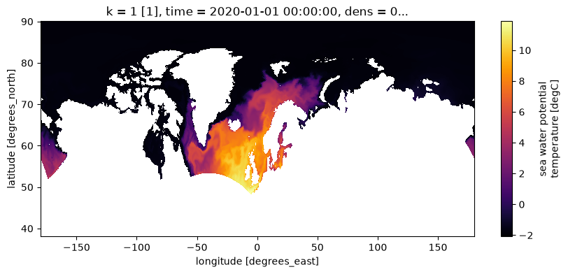
Chaining the two standalone pieces — horizontal then vertical — is exactly what regrid does by default. (Whether to run in this order or the reverse is a real choice, compared in the next section.)
# Chaining the standalone pieces == xhycom.regrid(ds, target=glorys, grid=grid):
ds_hv = xhycom.regrid_vertical(ds_h, depth=glorys["depth"].values)
ds_hv
<xarray.Dataset> Size: 20TB
Dimensions:     (time: 366, lat: 624, lon: 4320, ki: 51, depth: 50)
Coordinates:
  * time        (time) object 3kB 2020-01-01 00:00:00 ... 2020-12-31 00:00:00
  * lat         (lat) float32 2kB 38.08 38.17 38.25 38.33 ... 89.83 89.92 90.0
  * lon         (lon) float32 17kB -180.0 -179.9 -179.8 ... 179.8 179.8 179.9
  * ki          (ki) int64 408B 0 1 2 3 4 5 6 7 8 ... 42 43 44 45 46 47 48 49 50
  * depth       (depth) float64 400B 0.494 1.541 2.646 ... 5.275e+03 5.728e+03
Data variables: (12/82)
    montg1      (time, lat, lon) float64 8GB dask.array<chunksize=(1, 624, 4320), meta=np.ndarray>
    srfhgt      (time, lat, lon) float64 8GB dask.array<chunksize=(1, 624, 4320), meta=np.ndarray>
    oneta       (time, lat, lon) float64 8GB dask.array<chunksize=(1, 624, 4320), meta=np.ndarray>
    surflx      (time, lat, lon) float64 8GB dask.array<chunksize=(1, 624, 4320), meta=np.ndarray>
    wtrflx      (time, lat, lon) float64 8GB dask.array<chunksize=(1, 624, 4320), meta=np.ndarray>
    salflx      (time, lat, lon) float64 8GB dask.array<chunksize=(1, 624, 4320), meta=np.ndarray>
    ...          ...
    light_sw    (time, lat, lon, depth) float64 395GB dask.array<chunksize=(1, 624, 4320, 50), meta=np.ndarray>
    attenuat    (time, lat, lon, depth) float64 395GB dask.array<chunksize=(1, 624, 4320, 50), meta=np.ndarray>
    total_ch    (time, lat, lon, depth) float64 395GB dask.array<chunksize=(1, 624, 4320, 50), meta=np.ndarray>
    total_ca    (time, lat, lon, depth) float64 395GB dask.array<chunksize=(1, 624, 4320, 50), meta=np.ndarray>
    u-vel.      (time, lat, lon, depth) float64 395GB dask.array<chunksize=(1, 624, 4320, 50), meta=np.ndarray>
    v-vel.      (time, lat, lon, depth) float64 395GB dask.array<chunksize=(1, 624, 4320, 50), meta=np.ndarray>
Attributes:
    iversn:         23
    iexpt:          28
    yrflag:         3
    archive_type:   mean
regrid_method: conservative- time: 366
- lat: 624
- lon: 4320
- ki: 51
- depth: 50
- time(time)object2020-01-01 00:00:00 ... 2020-12-...
- long_name :
- time
- axis :
- T
array([cftime.DatetimeGregorian(2020, 1, 1, 0, 0, 0, 0, has_year_zero=False), cftime.DatetimeGregorian(2020, 1, 2, 0, 0, 0, 0, has_year_zero=False), cftime.DatetimeGregorian(2020, 1, 3, 0, 0, 0, 0, has_year_zero=False), ..., cftime.DatetimeGregorian(2020, 12, 29, 0, 0, 0, 0, has_year_zero=False), cftime.DatetimeGregorian(2020, 12, 30, 0, 0, 0, 0, has_year_zero=False), cftime.DatetimeGregorian(2020, 12, 31, 0, 0, 0, 0, has_year_zero=False)], shape=(366,), dtype=object) - lat(lat)float3238.08 38.17 38.25 ... 89.92 90.0
- standard_name :
- latitude
- units :
- degrees_north
array([38.083332, 38.166668, 38.25 , ..., 89.833336, 89.916664, 90. ], shape=(624,), dtype=float32) - lon(lon)float32-180.0 -179.9 ... 179.8 179.9
- standard_name :
- longitude
- units :
- degrees_east
array([-180. , -179.91667, -179.83333, ..., 179.75 , 179.83333, 179.91667], shape=(4320,), dtype=float32) - ki(ki)int640 1 2 3 4 5 6 ... 45 46 47 48 49 50
- long_name :
- layer interface index
- units :
- 1
- axis :
- Z
array([ 0, 1, 2, 3, 4, 5, 6, 7, 8, 9, 10, 11, 12, 13, 14, 15, 16, 17, 18, 19, 20, 21, 22, 23, 24, 25, 26, 27, 28, 29, 30, 31, 32, 33, 34, 35, 36, 37, 38, 39, 40, 41, 42, 43, 44, 45, 46, 47, 48, 49, 50]) - depth(depth)float640.494 1.541 ... 5.275e+03 5.728e+03
- long_name :
- depth
- units :
- m
- positive :
- down
- axis :
- Z
array([4.940250e-01, 1.541375e+00, 2.645669e+00, 3.819495e+00, 5.078224e+00,
       6.440614e+00, 7.929560e+00, 9.572997e+00, 1.140500e+01, 1.346714e+01,
       1.581007e+01, 1.849556e+01, 2.159882e+01, 2.521141e+01, 2.944473e+01,
       3.443415e+01, 4.034405e+01, 4.737369e+01, 5.576429e+01, 6.580727e+01,
       7.785385e+01, 9.232607e+01, 1.097293e+02, 1.306660e+02, 1.558507e+02,
       1.861256e+02, 2.224752e+02, 2.660403e+02, 3.181274e+02, 3.802130e+02,
       4.539377e+02, 5.410889e+02, 6.435668e+02, 7.633331e+02, 9.023393e+02,
       1.062440e+03, 1.245291e+03, 1.452251e+03, 1.684284e+03, 1.941893e+03,
       2.225078e+03, 2.533336e+03, 2.865703e+03, 3.220820e+03, 3.597032e+03,
       3.992484e+03, 4.405224e+03, 4.833291e+03, 5.274784e+03, 5.727917e+03])
- montg1(time, lat, lon)float64dask.array<chunksize=(1, 624, 4320), meta=np.ndarray>
- long_name :
- Montgomery potential
- units :
- m2 s-2
Array Chunk Bytes 7.35 GiB 20.57 MiB Shape (366, 624, 4320) (1, 624, 4320) Dask graph 366 chunks in 742 graph layers Data type float64 numpy.ndarray - srfhgt(time, lat, lon)float64dask.array<chunksize=(1, 624, 4320), meta=np.ndarray>
- long_name :
- sea surface height
- units :
- m
- comment :
- converted from Pa (factor 0.101978)
Array Chunk Bytes 7.35 GiB 20.57 MiB Shape (366, 624, 4320) (1, 624, 4320) Dask graph 366 chunks in 743 graph layers Data type float64 numpy.ndarray - oneta(time, lat, lon)float64dask.array<chunksize=(1, 624, 4320), meta=np.ndarray>
- long_name :
- free surface elevation
- units :
- m
Array Chunk Bytes 7.35 GiB 20.57 MiB Shape (366, 624, 4320) (1, 624, 4320) Dask graph 366 chunks in 742 graph layers Data type float64 numpy.ndarray - surflx(time, lat, lon)float64dask.array<chunksize=(1, 624, 4320), meta=np.ndarray>
- long_name :
- net surface heat flux
- units :
- W m-2
Array Chunk Bytes 7.35 GiB 20.57 MiB Shape (366, 624, 4320) (1, 624, 4320) Dask graph 366 chunks in 742 graph layers Data type float64 numpy.ndarray - wtrflx(time, lat, lon)float64dask.array<chunksize=(1, 624, 4320), meta=np.ndarray>
- long_name :
- net surface freshwater flux
- units :
- m s-1
Array Chunk Bytes 7.35 GiB 20.57 MiB Shape (366, 624, 4320) (1, 624, 4320) Dask graph 366 chunks in 742 graph layers Data type float64 numpy.ndarray - salflx(time, lat, lon)float64dask.array<chunksize=(1, 624, 4320), meta=np.ndarray>
- long_name :
- surface salt flux
- units :
- PSU m s-1
Array Chunk Bytes 7.35 GiB 20.57 MiB Shape (366, 624, 4320) (1, 624, 4320) Dask graph 366 chunks in 742 graph layers Data type float64 numpy.ndarray - bl_dpth(time, lat, lon)float64dask.array<chunksize=(1, 624, 4320), meta=np.ndarray>
- long_name :
- boundary layer depth
- units :
- m
- comment :
- converted from Pa (factor 0.000101978)
Array Chunk Bytes 7.35 GiB 20.57 MiB Shape (366, 624, 4320) (1, 624, 4320) Dask graph 366 chunks in 743 graph layers Data type float64 numpy.ndarray - mix_dpth(time, lat, lon)float64dask.array<chunksize=(1, 624, 4320), meta=np.ndarray>
- long_name :
- mixed layer depth
- units :
- m
- comment :
- converted from Pa (factor 0.000101978)
Array Chunk Bytes 7.35 GiB 20.57 MiB Shape (366, 624, 4320) (1, 624, 4320) Dask graph 366 chunks in 743 graph layers Data type float64 numpy.ndarray - tmix(time, lat, lon)float64dask.array<chunksize=(1, 624, 4320), meta=np.ndarray>
- long_name :
- mixed layer temperature
- units :
- degC
Array Chunk Bytes 7.35 GiB 20.57 MiB Shape (366, 624, 4320) (1, 624, 4320) Dask graph 366 chunks in 742 graph layers Data type float64 numpy.ndarray - smix(time, lat, lon)float64dask.array<chunksize=(1, 624, 4320), meta=np.ndarray>
- long_name :
- mixed layer salinity
- units :
- PSU
Array Chunk Bytes 7.35 GiB 20.57 MiB Shape (366, 624, 4320) (1, 624, 4320) Dask graph 366 chunks in 742 graph layers Data type float64 numpy.ndarray - thmix(time, lat, lon)float64dask.array<chunksize=(1, 624, 4320), meta=np.ndarray>
- long_name :
- mixed layer thickness
- units :
- m
- comment :
- converted from Pa (factor 0.000101978)
Array Chunk Bytes 7.35 GiB 20.57 MiB Shape (366, 624, 4320) (1, 624, 4320) Dask graph 366 chunks in 743 graph layers Data type float64 numpy.ndarray - kemix(time, lat, lon)float64dask.array<chunksize=(1, 624, 4320), meta=np.ndarray>
- long_name :
- mixed layer kinetic energy
- units :
- m2 s-2
Array Chunk Bytes 7.35 GiB 20.57 MiB Shape (366, 624, 4320) (1, 624, 4320) Dask graph 366 chunks in 742 graph layers Data type float64 numpy.ndarray - covice(time, lat, lon)float64dask.array<chunksize=(1, 624, 4320), meta=np.ndarray>
- long_name :
- sea ice coverage fraction
- units :
- 1
Array Chunk Bytes 7.35 GiB 20.57 MiB Shape (366, 624, 4320) (1, 624, 4320) Dask graph 366 chunks in 742 graph layers Data type float64 numpy.ndarray - thkice(time, lat, lon)float64dask.array<chunksize=(1, 624, 4320), meta=np.ndarray>
- long_name :
- sea ice thickness
- units :
- m
Array Chunk Bytes 7.35 GiB 20.57 MiB Shape (366, 624, 4320) (1, 624, 4320) Dask graph 366 chunks in 742 graph layers Data type float64 numpy.ndarray - temice(time, lat, lon)float64dask.array<chunksize=(1, 624, 4320), meta=np.ndarray>
- long_name :
- sea ice surface temperature
- units :
- degC
Array Chunk Bytes 7.35 GiB 20.57 MiB Shape (366, 624, 4320) (1, 624, 4320) Dask graph 366 chunks in 742 graph layers Data type float64 numpy.ndarray - kebtrop(time, lat, lon)float64dask.array<chunksize=(1, 624, 4320), meta=np.ndarray>
- long_name :
- barotropic kinetic energy
- units :
- m2 s-2
Array Chunk Bytes 7.35 GiB 20.57 MiB Shape (366, 624, 4320) (1, 624, 4320) Dask graph 366 chunks in 742 graph layers Data type float64 numpy.ndarray - light_pa(time, ki, lat, lon)float64dask.array<chunksize=(1, 51, 624, 4320), meta=np.ndarray>
- long_name :
- PAR irradiance
- units :
- W m-2
Array Chunk Bytes 374.90 GiB 1.02 GiB Shape (366, 51, 624, 4320) (1, 51, 624, 4320) Dask graph 366 chunks in 742 graph layers Data type float64 numpy.ndarray - ECO_sed4(time, lat, lon)float64dask.array<chunksize=(1, 624, 4320), meta=np.ndarray>
- long_name :
- sediment pool 4
- units :
- mmol m-2
Array Chunk Bytes 7.35 GiB 20.57 MiB Shape (366, 624, 4320) (1, 624, 4320) Dask graph 366 chunks in 742 graph layers Data type float64 numpy.ndarray - ECO_sed1(time, lat, lon)float64dask.array<chunksize=(1, 624, 4320), meta=np.ndarray>
- long_name :
- sediment pool 1
- units :
- mmol m-2
Array Chunk Bytes 7.35 GiB 20.57 MiB Shape (366, 624, 4320) (1, 624, 4320) Dask graph 366 chunks in 742 graph layers Data type float64 numpy.ndarray - ECO_sed2(time, lat, lon)float64dask.array<chunksize=(1, 624, 4320), meta=np.ndarray>
- long_name :
- sediment pool 2
- units :
- mmol m-2
Array Chunk Bytes 7.35 GiB 20.57 MiB Shape (366, 624, 4320) (1, 624, 4320) Dask graph 366 chunks in 742 graph layers Data type float64 numpy.ndarray - ECO_sed3(time, lat, lon)float64dask.array<chunksize=(1, 624, 4320), meta=np.ndarray>
- long_name :
- sediment pool 3
- units :
- mmol m-2
Array Chunk Bytes 7.35 GiB 20.57 MiB Shape (366, 624, 4320) (1, 624, 4320) Dask graph 366 chunks in 742 graph layers Data type float64 numpy.ndarray - CO2_fair(time, lat, lon)float64dask.array<chunksize=(1, 624, 4320), meta=np.ndarray>
- long_name :
- air-sea CO2 flux
- units :
- mmol C m-2 d-1
Array Chunk Bytes 7.35 GiB 20.57 MiB Shape (366, 624, 4320) (1, 624, 4320) Dask graph 366 chunks in 742 graph layers Data type float64 numpy.ndarray - CO2_wind(time, lat, lon)float64dask.array<chunksize=(1, 624, 4320), meta=np.ndarray>
- long_name :
- wind speed for gas exchange
- units :
- m s-1
Array Chunk Bytes 7.35 GiB 20.57 MiB Shape (366, 624, 4320) (1, 624, 4320) Dask graph 366 chunks in 742 graph layers Data type float64 numpy.ndarray - ECO_bots(time, lat, lon)float64dask.array<chunksize=(1, 624, 4320), meta=np.ndarray>
- long_name :
- bottom sediment flux
- units :
- 1
Array Chunk Bytes 7.35 GiB 20.57 MiB Shape (366, 624, 4320) (1, 624, 4320) Dask graph 366 chunks in 742 graph layers Data type float64 numpy.ndarray - surface__1(time, lat, lon)float64dask.array<chunksize=(1, 624, 4320), meta=np.ndarray>
Array Chunk Bytes 7.35 GiB 20.57 MiB Shape (366, 624, 4320) (1, 624, 4320) Dask graph 366 chunks in 742 graph layers Data type float64 numpy.ndarray - surface__2(time, lat, lon)float64dask.array<chunksize=(1, 624, 4320), meta=np.ndarray>
Array Chunk Bytes 7.35 GiB 20.57 MiB Shape (366, 624, 4320) (1, 624, 4320) Dask graph 366 chunks in 742 graph layers Data type float64 numpy.ndarray - u_btrop(time, lat, lon)float64dask.array<chunksize=(1, 624, 4320), meta=np.ndarray>
- long_name :
- eastward component of barotropic x velocity
- units :
- m s-1
- standard_name :
- eastward_sea_water_velocity
- comment :
- de-staggered to T-points and rotated to geographic axes
Array Chunk Bytes 7.35 GiB 20.57 MiB Shape (366, 624, 4320) (1, 624, 4320) Dask graph 366 chunks in 1493 graph layers Data type float64 numpy.ndarray - v_btrop(time, lat, lon)float64dask.array<chunksize=(1, 624, 4320), meta=np.ndarray>
- long_name :
- northward component of barotropic y velocity
- units :
- m s-1
- standard_name :
- northward_sea_water_velocity
- comment :
- de-staggered to T-points and rotated to geographic axes
Array Chunk Bytes 7.35 GiB 20.57 MiB Shape (366, 624, 4320) (1, 624, 4320) Dask graph 366 chunks in 1493 graph layers Data type float64 numpy.ndarray - umix(time, lat, lon)float64dask.array<chunksize=(1, 624, 4320), meta=np.ndarray>
- long_name :
- eastward component of mixed layer x velocity
- units :
- m s-1
- standard_name :
- eastward_sea_water_velocity
- comment :
- de-staggered to T-points and rotated to geographic axes
Array Chunk Bytes 7.35 GiB 20.57 MiB Shape (366, 624, 4320) (1, 624, 4320) Dask graph 366 chunks in 1493 graph layers Data type float64 numpy.ndarray - vmix(time, lat, lon)float64dask.array<chunksize=(1, 624, 4320), meta=np.ndarray>
- long_name :
- northward component of mixed layer y velocity
- units :
- m s-1
- standard_name :
- northward_sea_water_velocity
- comment :
- de-staggered to T-points and rotated to geographic axes
Array Chunk Bytes 7.35 GiB 20.57 MiB Shape (366, 624, 4320) (1, 624, 4320) Dask graph 366 chunks in 1493 graph layers Data type float64 numpy.ndarray - si_u(time, lat, lon)float64dask.array<chunksize=(1, 624, 4320), meta=np.ndarray>
- long_name :
- eastward component of sea ice x velocity
- units :
- m s-1
- standard_name :
- eastward_sea_water_velocity
- comment :
- de-staggered to T-points and rotated to geographic axes
Array Chunk Bytes 7.35 GiB 20.57 MiB Shape (366, 624, 4320) (1, 624, 4320) Dask graph 366 chunks in 1493 graph layers Data type float64 numpy.ndarray - si_v(time, lat, lon)float64dask.array<chunksize=(1, 624, 4320), meta=np.ndarray>
- long_name :
- northward component of sea ice y velocity
- units :
- m s-1
- standard_name :
- northward_sea_water_velocity
- comment :
- de-staggered to T-points and rotated to geographic axes
Array Chunk Bytes 7.35 GiB 20.57 MiB Shape (366, 624, 4320) (1, 624, 4320) Dask graph 366 chunks in 1493 graph layers Data type float64 numpy.ndarray - k.e.(time, lat, lon, depth)float64dask.array<chunksize=(1, 624, 4320, 50), meta=np.ndarray>
- long_name :
- kinetic energy
- units :
- m2 s-2
Array Chunk Bytes 367.54 GiB 1.00 GiB Shape (366, 624, 4320, 50) (1, 624, 4320, 50) Dask graph 366 chunks in 1507 graph layers Data type float64 numpy.ndarray - temp(time, lat, lon, depth)float64dask.array<chunksize=(1, 624, 4320, 50), meta=np.ndarray>
- long_name :
- sea water potential temperature
- units :
- degC
Array Chunk Bytes 367.54 GiB 1.00 GiB Shape (366, 624, 4320, 50) (1, 624, 4320, 50) Dask graph 366 chunks in 1507 graph layers Data type float64 numpy.ndarray - salin(time, lat, lon, depth)float64dask.array<chunksize=(1, 624, 4320, 50), meta=np.ndarray>
- long_name :
- sea water salinity
- units :
- PSU
Array Chunk Bytes 367.54 GiB 1.00 GiB Shape (366, 624, 4320, 50) (1, 624, 4320, 50) Dask graph 366 chunks in 1507 graph layers Data type float64 numpy.ndarray - density(time, lat, lon, depth)float64dask.array<chunksize=(1, 624, 4320, 50), meta=np.ndarray>
- long_name :
- sea water potential density (sigma-2)
- units :
- kg m-3
Array Chunk Bytes 367.54 GiB 1.00 GiB Shape (366, 624, 4320, 50) (1, 624, 4320, 50) Dask graph 366 chunks in 1507 graph layers Data type float64 numpy.ndarray - CO2_c(time, lat, lon, depth)float64dask.array<chunksize=(1, 624, 4320, 50), meta=np.ndarray>
- long_name :
- dissolved inorganic carbon
- units :
- mmol C m-3
Array Chunk Bytes 367.54 GiB 1.00 GiB Shape (366, 624, 4320, 50) (1, 624, 4320, 50) Dask graph 366 chunks in 1507 graph layers Data type float64 numpy.ndarray - CO2_TA(time, lat, lon, depth)float64dask.array<chunksize=(1, 624, 4320, 50), meta=np.ndarray>
- long_name :
- total alkalinity
- units :
- mmol eq m-3
Array Chunk Bytes 367.54 GiB 1.00 GiB Shape (366, 624, 4320, 50) (1, 624, 4320, 50) Dask graph 366 chunks in 1507 graph layers Data type float64 numpy.ndarray - ECO_no3(time, lat, lon, depth)float64dask.array<chunksize=(1, 624, 4320, 50), meta=np.ndarray>
- long_name :
- nitrate
- units :
- mmol N m-3
Array Chunk Bytes 367.54 GiB 1.00 GiB Shape (366, 624, 4320, 50) (1, 624, 4320, 50) Dask graph 366 chunks in 1507 graph layers Data type float64 numpy.ndarray - ECO_nh4(time, lat, lon, depth)float64dask.array<chunksize=(1, 624, 4320, 50), meta=np.ndarray>
- long_name :
- ammonium
- units :
- mmol N m-3
Array Chunk Bytes 367.54 GiB 1.00 GiB Shape (366, 624, 4320, 50) (1, 624, 4320, 50) Dask graph 366 chunks in 1507 graph layers Data type float64 numpy.ndarray - ECO_pho(time, lat, lon, depth)float64dask.array<chunksize=(1, 624, 4320, 50), meta=np.ndarray>
- long_name :
- phosphate
- units :
- mmol P m-3
Array Chunk Bytes 367.54 GiB 1.00 GiB Shape (366, 624, 4320, 50) (1, 624, 4320, 50) Dask graph 366 chunks in 1507 graph layers Data type float64 numpy.ndarray - ECO_sil(time, lat, lon, depth)float64dask.array<chunksize=(1, 624, 4320, 50), meta=np.ndarray>
- long_name :
- silicate
- units :
- mmol Si m-3
Array Chunk Bytes 367.54 GiB 1.00 GiB Shape (366, 624, 4320, 50) (1, 624, 4320, 50) Dask graph 366 chunks in 1507 graph layers Data type float64 numpy.ndarray - ECO_oxy(time, lat, lon, depth)float64dask.array<chunksize=(1, 624, 4320, 50), meta=np.ndarray>
- long_name :
- dissolved oxygen
- units :
- mmol O m-3
Array Chunk Bytes 367.54 GiB 1.00 GiB Shape (366, 624, 4320, 50) (1, 624, 4320, 50) Dask graph 366 chunks in 1507 graph layers Data type float64 numpy.ndarray - ECO_fla(time, lat, lon, depth)float64dask.array<chunksize=(1, 624, 4320, 50), meta=np.ndarray>
- long_name :
- flagellate carbon
- units :
- mmol C m-3
Array Chunk Bytes 367.54 GiB 1.00 GiB Shape (366, 624, 4320, 50) (1, 624, 4320, 50) Dask graph 366 chunks in 1507 graph layers Data type float64 numpy.ndarray - ECO_dia(time, lat, lon, depth)float64dask.array<chunksize=(1, 624, 4320, 50), meta=np.ndarray>
- long_name :
- diatom carbon
- units :
- mmol C m-3
Array Chunk Bytes 367.54 GiB 1.00 GiB Shape (366, 624, 4320, 50) (1, 624, 4320, 50) Dask graph 366 chunks in 1507 graph layers Data type float64 numpy.ndarray - ECO_ccl(time, lat, lon, depth)float64dask.array<chunksize=(1, 624, 4320, 50), meta=np.ndarray>
- long_name :
- coccolithophore carbon
- units :
- mmol C m-3
Array Chunk Bytes 367.54 GiB 1.00 GiB Shape (366, 624, 4320, 50) (1, 624, 4320, 50) Dask graph 366 chunks in 1507 graph layers Data type float64 numpy.ndarray - ECO_cclc(time, lat, lon, depth)float64dask.array<chunksize=(1, 624, 4320, 50), meta=np.ndarray>
- long_name :
- coccolithophore calcite carbon
- units :
- mmol C m-3
Array Chunk Bytes 367.54 GiB 1.00 GiB Shape (366, 624, 4320, 50) (1, 624, 4320, 50) Dask graph 366 chunks in 1507 graph layers Data type float64 numpy.ndarray - ECO_caco(time, lat, lon, depth)float64dask.array<chunksize=(1, 624, 4320, 50), meta=np.ndarray>
- long_name :
- particulate inorganic carbon (calcite)
- units :
- mmol C m-3
Array Chunk Bytes 367.54 GiB 1.00 GiB Shape (366, 624, 4320, 50) (1, 624, 4320, 50) Dask graph 366 chunks in 1507 graph layers Data type float64 numpy.ndarray - ECO_diac(time, lat, lon, depth)float64dask.array<chunksize=(1, 624, 4320, 50), meta=np.ndarray>
- long_name :
- diatom calcite carbon
- units :
- mmol C m-3
Array Chunk Bytes 367.54 GiB 1.00 GiB Shape (366, 624, 4320, 50) (1, 624, 4320, 50) Dask graph 366 chunks in 1507 graph layers Data type float64 numpy.ndarray - ECO_flac(time, lat, lon, depth)float64dask.array<chunksize=(1, 624, 4320, 50), meta=np.ndarray>
- long_name :
- flagellate calcite carbon
- units :
- mmol C m-3
Array Chunk Bytes 367.54 GiB 1.00 GiB Shape (366, 624, 4320, 50) (1, 624, 4320, 50) Dask graph 366 chunks in 1507 graph layers Data type float64 numpy.ndarray - ECO_micr(time, lat, lon, depth)float64dask.array<chunksize=(1, 624, 4320, 50), meta=np.ndarray>
- long_name :
- microzooplankton carbon
- units :
- mmol C m-3
Array Chunk Bytes 367.54 GiB 1.00 GiB Shape (366, 624, 4320, 50) (1, 624, 4320, 50) Dask graph 366 chunks in 1507 graph layers Data type float64 numpy.ndarray - ECO_meso(time, lat, lon, depth)float64dask.array<chunksize=(1, 624, 4320, 50), meta=np.ndarray>
- long_name :
- mesozooplankton carbon
- units :
- mmol C m-3
Array Chunk Bytes 367.54 GiB 1.00 GiB Shape (366, 624, 4320, 50) (1, 624, 4320, 50) Dask graph 366 chunks in 1507 graph layers Data type float64 numpy.ndarray - ECO_det(time, lat, lon, depth)float64dask.array<chunksize=(1, 624, 4320, 50), meta=np.ndarray>
- long_name :
- detritus carbon
- units :
- mmol C m-3
Array Chunk Bytes 367.54 GiB 1.00 GiB Shape (366, 624, 4320, 50) (1, 624, 4320, 50) Dask graph 366 chunks in 1507 graph layers Data type float64 numpy.ndarray - ECO_opa(time, lat, lon, depth)float64dask.array<chunksize=(1, 624, 4320, 50), meta=np.ndarray>
- long_name :
- opal (biogenic silica)
- units :
- mmol Si m-3
Array Chunk Bytes 367.54 GiB 1.00 GiB Shape (366, 624, 4320, 50) (1, 624, 4320, 50) Dask graph 366 chunks in 1507 graph layers Data type float64 numpy.ndarray - ECO_dom(time, lat, lon, depth)float64dask.array<chunksize=(1, 624, 4320, 50), meta=np.ndarray>
- long_name :
- dissolved organic matter carbon
- units :
- mmol C m-3
Array Chunk Bytes 367.54 GiB 1.00 GiB Shape (366, 624, 4320, 50) (1, 624, 4320, 50) Dask graph 366 chunks in 1507 graph layers Data type float64 numpy.ndarray - ECO_dsnk(time, lat, lon, depth)float64dask.array<chunksize=(1, 624, 4320, 50), meta=np.ndarray>
- long_name :
- detritus sinking flux
- units :
- mmol C m-2 s-1
Array Chunk Bytes 367.54 GiB 1.00 GiB Shape (366, 624, 4320, 50) (1, 624, 4320, 50) Dask graph 366 chunks in 1507 graph layers Data type float64 numpy.ndarray - CO2_pH(time, lat, lon, depth)float64dask.array<chunksize=(1, 624, 4320, 50), meta=np.ndarray>
- long_name :
- seawater pH
- units :
- 1
Array Chunk Bytes 367.54 GiB 1.00 GiB Shape (366, 624, 4320, 50) (1, 624, 4320, 50) Dask graph 366 chunks in 1507 graph layers Data type float64 numpy.ndarray - CO2_pCO2(time, lat, lon, depth)float64dask.array<chunksize=(1, 624, 4320, 50), meta=np.ndarray>
- long_name :
- partial pressure of CO2
- units :
- uatm
Array Chunk Bytes 367.54 GiB 1.00 GiB Shape (366, 624, 4320, 50) (1, 624, 4320, 50) Dask graph 366 chunks in 1507 graph layers Data type float64 numpy.ndarray - CO2_Carb_1(time, lat, lon, depth)float64dask.array<chunksize=(1, 624, 4320, 50), meta=np.ndarray>
- long_name :
- carbonate concentration
- units :
- mmol C m-3
Array Chunk Bytes 367.54 GiB 1.00 GiB Shape (366, 624, 4320, 50) (1, 624, 4320, 50) Dask graph 366 chunks in 1507 graph layers Data type float64 numpy.ndarray - CO2_BiCa(time, lat, lon, depth)float64dask.array<chunksize=(1, 624, 4320, 50), meta=np.ndarray>
- long_name :
- bicarbonate concentration
- units :
- mmol C m-3
Array Chunk Bytes 367.54 GiB 1.00 GiB Shape (366, 624, 4320, 50) (1, 624, 4320, 50) Dask graph 366 chunks in 1507 graph layers Data type float64 numpy.ndarray - CO2_Carb_2(time, lat, lon, depth)float64dask.array<chunksize=(1, 624, 4320, 50), meta=np.ndarray>
- long_name :
- carbonate concentration
- units :
- mmol C m-3
Array Chunk Bytes 367.54 GiB 1.00 GiB Shape (366, 624, 4320, 50) (1, 624, 4320, 50) Dask graph 366 chunks in 1507 graph layers Data type float64 numpy.ndarray - CO2_Om_c(time, lat, lon, depth)float64dask.array<chunksize=(1, 624, 4320, 50), meta=np.ndarray>
- long_name :
- calcite saturation state (Omega)
- units :
- 1
Array Chunk Bytes 367.54 GiB 1.00 GiB Shape (366, 624, 4320, 50) (1, 624, 4320, 50) Dask graph 366 chunks in 1507 graph layers Data type float64 numpy.ndarray - CO2_Om_a(time, lat, lon, depth)float64dask.array<chunksize=(1, 624, 4320, 50), meta=np.ndarray>
- long_name :
- aragonite saturation state (Omega)
- units :
- 1
Array Chunk Bytes 367.54 GiB 1.00 GiB Shape (366, 624, 4320, 50) (1, 624, 4320, 50) Dask graph 366 chunks in 1507 graph layers Data type float64 numpy.ndarray - ECO_prim(time, lat, lon, depth)float64dask.array<chunksize=(1, 624, 4320, 50), meta=np.ndarray>
- long_name :
- primary production
- units :
- mmol C m-3 s-1
Array Chunk Bytes 367.54 GiB 1.00 GiB Shape (366, 624, 4320, 50) (1, 624, 4320, 50) Dask graph 366 chunks in 1507 graph layers Data type float64 numpy.ndarray - ECO_secp(time, lat, lon, depth)float64dask.array<chunksize=(1, 624, 4320, 50), meta=np.ndarray>
- long_name :
- secondary production
- units :
- mmol C m-3 s-1
Array Chunk Bytes 367.54 GiB 1.00 GiB Shape (366, 624, 4320, 50) (1, 624, 4320, 50) Dask graph 366 chunks in 1507 graph layers Data type float64 numpy.ndarray - ECO_netp(time, lat, lon, depth)float64dask.array<chunksize=(1, 624, 4320, 50), meta=np.ndarray>
- long_name :
- net primary production
- units :
- mmol C m-3 s-1
Array Chunk Bytes 367.54 GiB 1.00 GiB Shape (366, 624, 4320, 50) (1, 624, 4320, 50) Dask graph 366 chunks in 1507 graph layers Data type float64 numpy.ndarray - ECO_parm(time, lat, lon, depth)float64dask.array<chunksize=(1, 624, 4320, 50), meta=np.ndarray>
- long_name :
- BGC parameter field
- units :
- 1
Array Chunk Bytes 367.54 GiB 1.00 GiB Shape (366, 624, 4320, 50) (1, 624, 4320, 50) Dask graph 366 chunks in 1507 graph layers Data type float64 numpy.ndarray - ECO_Nlim(time, lat, lon, depth)float64dask.array<chunksize=(1, 624, 4320, 50), meta=np.ndarray>
- long_name :
- nitrogen limitation factor
- units :
- 1
Array Chunk Bytes 367.54 GiB 1.00 GiB Shape (366, 624, 4320, 50) (1, 624, 4320, 50) Dask graph 366 chunks in 1507 graph layers Data type float64 numpy.ndarray - ECO_Plim(time, lat, lon, depth)float64dask.array<chunksize=(1, 624, 4320, 50), meta=np.ndarray>
- long_name :
- phosphorus limitation factor
- units :
- 1
Array Chunk Bytes 367.54 GiB 1.00 GiB Shape (366, 624, 4320, 50) (1, 624, 4320, 50) Dask graph 366 chunks in 1507 graph layers Data type float64 numpy.ndarray - ECO_Slim(time, lat, lon, depth)float64dask.array<chunksize=(1, 624, 4320, 50), meta=np.ndarray>
- long_name :
- silicate limitation factor
- units :
- 1
Array Chunk Bytes 367.54 GiB 1.00 GiB Shape (366, 624, 4320, 50) (1, 624, 4320, 50) Dask graph 366 chunks in 1507 graph layers Data type float64 numpy.ndarray - ECO_Llim(time, lat, lon, depth)float64dask.array<chunksize=(1, 624, 4320, 50), meta=np.ndarray>
- long_name :
- light limitation factor
- units :
- 1
Array Chunk Bytes 367.54 GiB 1.00 GiB Shape (366, 624, 4320, 50) (1, 624, 4320, 50) Dask graph 366 chunks in 1507 graph layers Data type float64 numpy.ndarray - ECO_deni(time, lat, lon, depth)float64dask.array<chunksize=(1, 624, 4320, 50), meta=np.ndarray>
- long_name :
- denitrification
- units :
- mmol N m-3 s-1
Array Chunk Bytes 367.54 GiB 1.00 GiB Shape (366, 624, 4320, 50) (1, 624, 4320, 50) Dask graph 366 chunks in 1507 graph layers Data type float64 numpy.ndarray - ECO_snks(time, lat, lon, depth)float64dask.array<chunksize=(1, 624, 4320, 50), meta=np.ndarray>
- long_name :
- sinking rate
- units :
- m d-1
Array Chunk Bytes 367.54 GiB 1.00 GiB Shape (366, 624, 4320, 50) (1, 624, 4320, 50) Dask graph 366 chunks in 1507 graph layers Data type float64 numpy.ndarray - ECO_c2ch_1(time, lat, lon, depth)float64dask.array<chunksize=(1, 624, 4320, 50), meta=np.ndarray>
- long_name :
- carbon to chlorophyll ratio
- units :
- g C g-1 Chl
Array Chunk Bytes 367.54 GiB 1.00 GiB Shape (366, 624, 4320, 50) (1, 624, 4320, 50) Dask graph 366 chunks in 1507 graph layers Data type float64 numpy.ndarray - ECO_c2ch_2(time, lat, lon, depth)float64dask.array<chunksize=(1, 624, 4320, 50), meta=np.ndarray>
- long_name :
- carbon to chlorophyll ratio
- units :
- g C g-1 Chl
Array Chunk Bytes 367.54 GiB 1.00 GiB Shape (366, 624, 4320, 50) (1, 624, 4320, 50) Dask graph 366 chunks in 1507 graph layers Data type float64 numpy.ndarray - ECO_c2ch_3(time, lat, lon, depth)float64dask.array<chunksize=(1, 624, 4320, 50), meta=np.ndarray>
- long_name :
- carbon to chlorophyll ratio
- units :
- g C g-1 Chl
Array Chunk Bytes 367.54 GiB 1.00 GiB Shape (366, 624, 4320, 50) (1, 624, 4320, 50) Dask graph 366 chunks in 1507 graph layers Data type float64 numpy.ndarray - light_sw(time, lat, lon, depth)float64dask.array<chunksize=(1, 624, 4320, 50), meta=np.ndarray>
- long_name :
- shortwave irradiance in water
- units :
- W m-2
Array Chunk Bytes 367.54 GiB 1.00 GiB Shape (366, 624, 4320, 50) (1, 624, 4320, 50) Dask graph 366 chunks in 1507 graph layers Data type float64 numpy.ndarray - attenuat(time, lat, lon, depth)float64dask.array<chunksize=(1, 624, 4320, 50), meta=np.ndarray>
- long_name :
- light attenuation coefficient
- units :
- m-1
Array Chunk Bytes 367.54 GiB 1.00 GiB Shape (366, 624, 4320, 50) (1, 624, 4320, 50) Dask graph 366 chunks in 1507 graph layers Data type float64 numpy.ndarray - total_ch(time, lat, lon, depth)float64dask.array<chunksize=(1, 624, 4320, 50), meta=np.ndarray>
- long_name :
- total chlorophyll
- units :
- mg Chl m-3
Array Chunk Bytes 367.54 GiB 1.00 GiB Shape (366, 624, 4320, 50) (1, 624, 4320, 50) Dask graph 366 chunks in 1507 graph layers Data type float64 numpy.ndarray - total_ca(time, lat, lon, depth)float64dask.array<chunksize=(1, 624, 4320, 50), meta=np.ndarray>
- long_name :
- total carbon
- units :
- mmol C m-3
Array Chunk Bytes 367.54 GiB 1.00 GiB Shape (366, 624, 4320, 50) (1, 624, 4320, 50) Dask graph 366 chunks in 1507 graph layers Data type float64 numpy.ndarray - u-vel.(time, lat, lon, depth)float64dask.array<chunksize=(1, 624, 4320, 50), meta=np.ndarray>
- long_name :
- eastward component of sea water x velocity
- units :
- m s-1
- hycom_velocity :
- total
- comment :
- de-staggered to T-points and rotated to geographic axes
- standard_name :
- eastward_sea_water_velocity
Array Chunk Bytes 367.54 GiB 1.00 GiB Shape (366, 624, 4320, 50) (1, 624, 4320, 50) Dask graph 366 chunks in 2258 graph layers Data type float64 numpy.ndarray - v-vel.(time, lat, lon, depth)float64dask.array<chunksize=(1, 624, 4320, 50), meta=np.ndarray>
- long_name :
- northward component of sea water y velocity
- units :
- m s-1
- hycom_velocity :
- total
- comment :
- de-staggered to T-points and rotated to geographic axes
- standard_name :
- northward_sea_water_velocity
Array Chunk Bytes 367.54 GiB 1.00 GiB Shape (366, 624, 4320, 50) (1, 624, 4320, 50) Dask graph 366 chunks in 2258 graph layers Data type float64 numpy.ndarray
- iversn :
- 23
- iexpt :
- 28
- yrflag :
- 3
- archive_type :
- mean
- regrid_method :
- conservative
Which regridding order? Mix along isopycnals#
regrid runs the lateral and vertical steps in sequence, and the order is not neutral. HYCOM’s hybrid layers are isopycnals in the stratified interior, and temperature and salinity mix along isopycnals — so where the lateral averaging happens matters:
order="horizontal_first"(default) blends along the native layers → mixes same-density water, preserving water masses and the T–S relationship.order="vertical_first"blends at constant depth → where isopycnals tilt (fronts, slopes) it mixes across density surfaces and smears water masses, though it resolves more cells on shelves and slopes.
Both conserve the global integral; they differ locally. Run both and compare:
g_hf = xhycom.regrid(ds, target=glorys, grid=grid, order="horizontal_first")
g_vf = xhycom.regrid(ds, target=glorys, grid=grid, order="vertical_first")
# extra ocean cells the depth-first order resolves near topography:
int(np.isfinite(g_vf["temp"]).isel(time=0).sum() - np.isfinite(g_hf["temp"]).isel(time=0).sum())
128308
The two agree across the smooth interior but diverge along fronts and topography. A meridional section of the difference shows constant-depth averaging mixing across tilted isopycnals — the dipoles sit on sloping density surfaces:
temp_vf = g_vf["temp"].isel(time=0).sel(lon=0, method="nearest")
temp_hf = g_hf["temp"].isel(time=0).sel(lon=0, method="nearest")
fig, axs = plt.subplots(1, 3, figsize=(25, 4))

temp_vf.plot(cmap="inferno", x="lat", y="depth", center=False, yincrease=False, ax=axs[0])
temp_hf.plot(cmap="inferno", x="lat", y="depth", center=False, yincrease=False, ax=axs[1])
(temp_vf - temp_hf).plot(x="lat", y="depth", vmin=-0.3, vmax=0.3, cmap="RdBu_r", center=0, yincrease=False, ax=axs[2])

for ax in axs:
    ax.set_xlim(50, None)      # latitude > 50
    ax.set_ylim(4200, None)    # depth < 4200 (see note below)

Recommendation: horizontal_first#
For temperature, salinity, and any water-mass analysis, use horizontal_first (the default) — it averages the way tracers actually mix. Reach for vertical_first only when geometric fidelity to a z-level product near topography outweighs water-mass integrity.
|
|
|
|---|---|---|
Lateral averaging |
along native isopycnal layers |
at constant depth |
Water masses / T–S |
preserved |
smeared across tilted isopycnals |
Shelf / slope coverage |
good |
best (per-column bathymetry) |
Global integral |
conserved |
conserved |
Use when |
T/S & water-mass budgets (most cases) |
matching z-level geometry near topography |
Method options#
Argument |
Default |
Alternatives |
|---|---|---|
|
|
|
|
|
|
Conservative (default) conserves area / depth integrals — use for budgets and fluxes. Horizontal needs source cell corners, so pass
grid=.Bilinear / linear interpolate point values — smoother, no
qlon/qlatneeded.Target mask — when
target=carries amask, its land points become NaN; disable withapply_target_mask=False.
The regridding is conservative#
Vertical — the transform thickness-weights each field, so a column’s depth integral (e.g. heat content \(\int T\,dz\)) is preserved.
zlev = np.arange(2.0, 6500, 4.0)
ds_z = xhycom.regrid_vertical(ds, depth=zlev)                 # conservative (default)
# Column integral ∫T dz on native hybrid layers vs on z-levels (one snapshot):
native  = (ds["temp"] * ds["thknss"]).isel(time=0).sum("k")   # hybrid layers
on_zlev = (ds_z["temp"] * 4.0).isel(time=0).sum("depth")      # z-levels (Δz = 4 m)
fig, axs = plt.subplots(1, 3, figsize=(20, 5))

native.plot(ax=axs[0])
on_zlev.plot(ax=axs[1])
(native - on_zlev).plot(ax=axs[2])
<matplotlib.collections.QuadMesh at 0x14d75c196850>
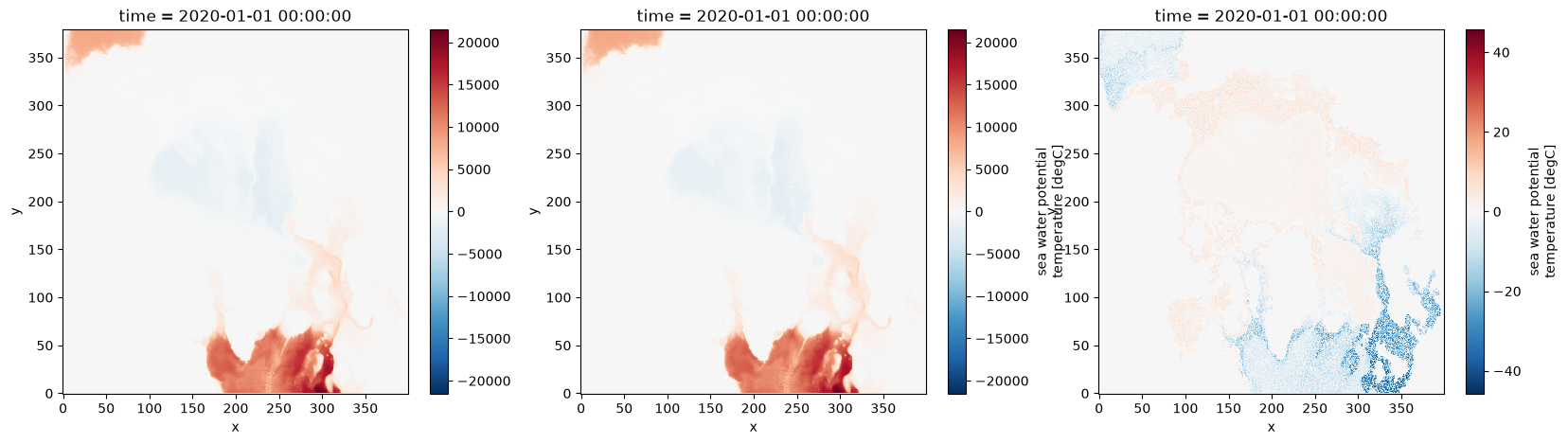
The absolute difference between the integral computed on native hybrid layers and on regridded z-levels is orders of magnitude smaller than the signal (compare first and second amplitudes versus the third).
Horizontal — conservative remapping reproduces a uniform field exactly (a defining property), so it conserves the area integral. Regrid a field of ones and map the deviation from 1 — it sits at machine precision (\(\sim 10^{-12}\)):
ones = ds[["temp"]].isel(time=0).copy()
ones["temp"] = xr.ones_like(ones["temp"])
out = xhycom.regrid_horizontal(ones, target=glorys, grid=grid, apply_target_mask=False)        # conservative (default)
# A uniform field must remap back to 1 everywhere — deviation is at machine precision:
(out["temp"].isel(k=0) - 1).plot(robust=True)                 # ~1e-12
<matplotlib.collections.QuadMesh at 0x14d4f47aed50>
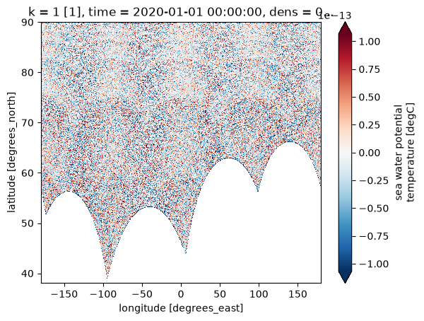
Velocities are rotated to east/north#
HYCOM stores velocities on a staggered Arakawa C-grid, with components along the model grid axes: u-vel. runs along the grid’s x-direction and v-vel. along y. On a curvilinear grid those axes are not east/north — they rotate across the domain (sharply near the grid’s poles). regrid / regrid_horizontal de-stagger the components to the T-points and rotate them onto the true geographic axes using the grid angle pang, so the output u-vel. / v-vel. are genuinely eastward / northward.
First, the native components along the model axes:
# Native components, plotted on their own staggered lon/lat — along the model axes.
fig, axs = plt.subplots(1, 2, figsize=(14, 4))
ds["u-vel."].isel(time=0, k=0).plot(ax=axs[0], cmap="RdBu_r", center=0)
ds["v-vel."].isel(time=0, k=0).plot(ax=axs[1], cmap="RdBu_r", center=0)
axs[0].set_title("native u-vel. — along model x-axis")
axs[1].set_title("native v-vel. — along model y-axis")
fig.tight_layout()
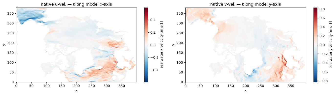
After regridding, u-vel. / v-vel. carry standard_name = eastward/northward_sea_water_velocity (and a comment recording the de-stagger and rotation). The real test that the rotation is physical — not just a relabel — is that on the shared GLORYS grid they line up with GLORYS’s own eastward (uo) / northward (vo) velocities:
# Surface velocities on the shared GLORYS grid.
hu = ds_g["u-vel."].isel(time=0, depth=0).compute()
hv = ds_g["v-vel."].isel(time=0, depth=0).compute()
gu = glorys_data["uo"].isel(time=0, depth=0)
gv = glorys_data["vo"].isel(time=0, depth=0)
fig, axs = plt.subplots(2, 2, figsize=(22, 8))
kw = dict(robust=True, cmap="RdBu_r", center=0)

hu.plot(ax=axs[0, 0], **kw)
gu.plot(ax=axs[0, 1], **kw)
hv.plot(ax=axs[1, 0], **kw)
gv.plot(ax=axs[1, 1], **kw)

titles = [["HYCOM eastward (u-vel.)", "GLORYS eastward (uo)"],
          ["HYCOM northward (v-vel.)", "GLORYS northward (vo)"]]

for r in range(2):
    for c in range(2):
        axs[r][c].set_title(titles[r][c])
fig.tight_layout()


for ax in axs.flatten():
    ax.set_ylim(50, None)      # latitude > 50
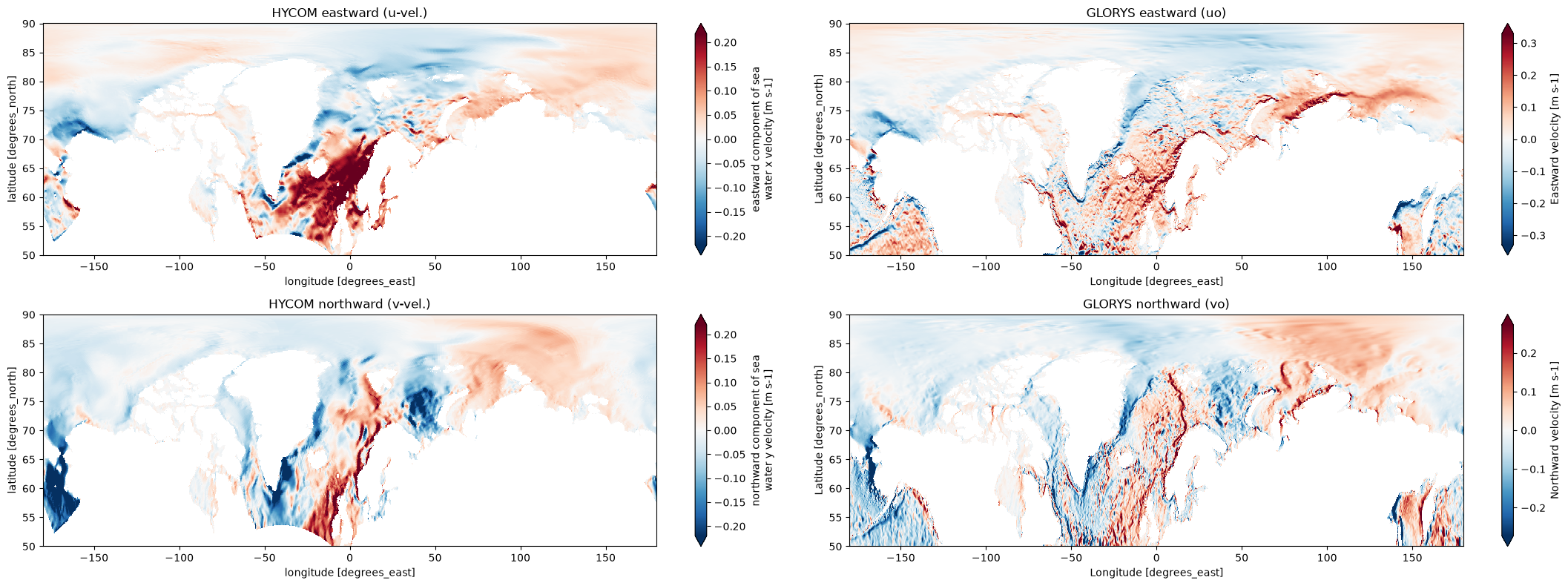
The GLORYS reanalysis shows substantially more mesoscale eddy activity than the HYCOM TOPAZ2 simulation due to its higher spatial resolution. Nevertheless, the large-scale velocity patterns and flow directions remain consistent between the two (compare left and right panels), confirming that xhycom performs the velocity rotation via .regrid and .regrid_horizontal correctly.
Caching the regrid weights#
Since the weights depend only on the grids, you can build them once and reuse them. Pass weights=True to cache the weight matrix to disk; later regrids of other files (or other runs in the same session) read it back instead of regenerating it.
The cache is keyed by grid geometry — the source idm/jdm and lon/lat extent (straight from regional.grid) plus the GLORYS shape/extent — so TP0/TP2/TP5 × target × method each get their own file under $XHYCOM_CACHE_DIR (default ~/.cache/xhycom/regrid_weights). Point XHYCOM_CACHE_DIR at project or scratch space to share weights across jobs.
import os

# Where to cache the xESMF weights. Set this *before* the first weights=True call.
os.environ["XHYCOM_CACHE_DIR"] = f"/cluster/projects/nn2993k/{os.environ['USER']}/.xhycom-cache-dir"
# First call: build the weights and write them to the cache.
%time ds_g = xhycom.regrid(ds, target=glorys, grid=grid, weights=True)
CPU times: user 49 s, sys: 7.13 s, total: 56.1 s
Wall time: 56.5 s
Re-running with the same grids reads the weights back from disk instead of regenerating them. Constructing the regrid is then cheap, and the field values stay lazy — weight generation is the only eager step; the actual remap streams per time chunk when you load.
call |
weight matrix |
field application |
|---|---|---|
first ( |
built once, written to cache |
lazy, per time chunk |
later files / sessions |
read from cache |
lazy, per time chunk |
# Second call reuses the cached weights; the result is dask-backed (lazy).
%time ds_g = xhycom.regrid(ds, target=glorys, grid=grid, weights=True)
ds_g # repr shows dask chunks — nothing computed yet
CPU times: user 25.4 s, sys: 7.11 s, total: 32.5 s
Wall time: 32.7 s
<xarray.Dataset> Size: 52TB
Dimensions:     (time: 366, lat: 624, lon: 4320, depth: 50, ki: 51)
Coordinates:
  * time        (time) object 3kB 2020-01-01 00:00:00 ... 2020-12-31 00:00:00
  * lat         (lat) float32 2kB 38.08 38.17 38.25 38.33 ... 89.83 89.92 90.0
  * lon         (lon) float32 17kB -180.0 -179.9 -179.8 ... 179.8 179.8 179.9
  * depth       (depth) float64 400B 0.494 1.541 2.646 ... 5.275e+03 5.728e+03
  * ki          (ki) int64 408B 0 1 2 3 4 5 6 7 8 ... 42 43 44 45 46 47 48 49 50
Data variables: (12/82)
    montg1      (time, lat, lon, depth) float64 395GB dask.array<chunksize=(1, 624, 4320, 50), meta=np.ndarray>
    srfhgt      (time, lat, lon, depth) float64 395GB dask.array<chunksize=(1, 624, 4320, 50), meta=np.ndarray>
    oneta       (time, lat, lon, depth) float64 395GB dask.array<chunksize=(1, 624, 4320, 50), meta=np.ndarray>
    surflx      (time, lat, lon, depth) float64 395GB dask.array<chunksize=(1, 624, 4320, 50), meta=np.ndarray>
    wtrflx      (time, lat, lon, depth) float64 395GB dask.array<chunksize=(1, 624, 4320, 50), meta=np.ndarray>
    salflx      (time, lat, lon, depth) float64 395GB dask.array<chunksize=(1, 624, 4320, 50), meta=np.ndarray>
    ...          ...
    light_sw    (time, lat, lon, depth) float64 395GB dask.array<chunksize=(1, 624, 4320, 50), meta=np.ndarray>
    attenuat    (time, lat, lon, depth) float64 395GB dask.array<chunksize=(1, 624, 4320, 50), meta=np.ndarray>
    total_ch    (time, lat, lon, depth) float64 395GB dask.array<chunksize=(1, 624, 4320, 50), meta=np.ndarray>
    total_ca    (time, lat, lon, depth) float64 395GB dask.array<chunksize=(1, 624, 4320, 50), meta=np.ndarray>
    u-vel.      (time, lat, lon, depth) float64 395GB dask.array<chunksize=(1, 624, 4320, 50), meta=np.ndarray>
    v-vel.      (time, lat, lon, depth) float64 395GB dask.array<chunksize=(1, 624, 4320, 50), meta=np.ndarray>
Attributes:
    iversn:         23
    iexpt:          28
    yrflag:         3
    archive_type:   mean
regrid_method: conservative- time: 366
- lat: 624
- lon: 4320
- depth: 50
- ki: 51
- time(time)object2020-01-01 00:00:00 ... 2020-12-...
- long_name :
- time
- axis :
- T
array([cftime.DatetimeGregorian(2020, 1, 1, 0, 0, 0, 0, has_year_zero=False), cftime.DatetimeGregorian(2020, 1, 2, 0, 0, 0, 0, has_year_zero=False), cftime.DatetimeGregorian(2020, 1, 3, 0, 0, 0, 0, has_year_zero=False), ..., cftime.DatetimeGregorian(2020, 12, 29, 0, 0, 0, 0, has_year_zero=False), cftime.DatetimeGregorian(2020, 12, 30, 0, 0, 0, 0, has_year_zero=False), cftime.DatetimeGregorian(2020, 12, 31, 0, 0, 0, 0, has_year_zero=False)], shape=(366,), dtype=object) - lat(lat)float3238.08 38.17 38.25 ... 89.92 90.0
- standard_name :
- latitude
- units :
- degrees_north
array([38.083332, 38.166668, 38.25 , ..., 89.833336, 89.916664, 90. ], shape=(624,), dtype=float32) - lon(lon)float32-180.0 -179.9 ... 179.8 179.9
- standard_name :
- longitude
- units :
- degrees_east
array([-180. , -179.91667, -179.83333, ..., 179.75 , 179.83333, 179.91667], shape=(4320,), dtype=float32) - depth(depth)float640.494 1.541 ... 5.275e+03 5.728e+03
- long_name :
- depth
- units :
- m
- positive :
- down
- axis :
- Z
array([4.940250e-01, 1.541375e+00, 2.645669e+00, 3.819495e+00, 5.078224e+00, 6.440614e+00, 7.929560e+00, 9.572997e+00, 1.140500e+01, 1.346714e+01, 1.581007e+01, 1.849556e+01, 2.159882e+01, 2.521141e+01, 2.944473e+01, 3.443415e+01, 4.034405e+01, 4.737369e+01, 5.576429e+01, 6.580727e+01, 7.785385e+01, 9.232607e+01, 1.097293e+02, 1.306660e+02, 1.558507e+02, 1.861256e+02, 2.224752e+02, 2.660403e+02, 3.181274e+02, 3.802130e+02, 4.539377e+02, 5.410889e+02, 6.435668e+02, 7.633331e+02, 9.023393e+02, 1.062440e+03, 1.245291e+03, 1.452251e+03, 1.684284e+03, 1.941893e+03, 2.225078e+03, 2.533336e+03, 2.865703e+03, 3.220820e+03, 3.597032e+03, 3.992484e+03, 4.405224e+03, 4.833291e+03, 5.274784e+03, 5.727917e+03]) - ki(ki)int640 1 2 3 4 5 6 ... 45 46 47 48 49 50
- long_name :
- layer interface index
- units :
- 1
- axis :
- Z
array([ 0,  1,  2,  3,  4,  5,  6,  7,  8,  9, 10, 11, 12, 13, 14, 15, 16, 17,
       18, 19, 20, 21, 22, 23, 24, 25, 26, 27, 28, 29, 30, 31, 32, 33, 34, 35,
       36, 37, 38, 39, 40, 41, 42, 43, 44, 45, 46, 47, 48, 49, 50])
- montg1(time, lat, lon, depth)float64dask.array<chunksize=(1, 624, 4320, 50), meta=np.ndarray>
- long_name :
- Montgomery potential
- units :
- m2 s-2
Array Chunk Bytes 367.54 GiB 1.00 GiB Shape (366, 624, 4320, 50) (1, 624, 4320, 50) Dask graph 366 chunks in 743 graph layers Data type float64 numpy.ndarray - srfhgt(time, lat, lon, depth)float64dask.array<chunksize=(1, 624, 4320, 50), meta=np.ndarray>
- long_name :
- sea surface height
- units :
- m
- comment :
- converted from Pa (factor 0.101978)
Array Chunk Bytes 367.54 GiB 1.00 GiB Shape (366, 624, 4320, 50) (1, 624, 4320, 50) Dask graph 366 chunks in 744 graph layers Data type float64 numpy.ndarray - oneta(time, lat, lon, depth)float64dask.array<chunksize=(1, 624, 4320, 50), meta=np.ndarray>
- long_name :
- free surface elevation
- units :
- m
Array Chunk Bytes 367.54 GiB 1.00 GiB Shape (366, 624, 4320, 50) (1, 624, 4320, 50) Dask graph 366 chunks in 743 graph layers Data type float64 numpy.ndarray - surflx(time, lat, lon, depth)float64dask.array<chunksize=(1, 624, 4320, 50), meta=np.ndarray>
- long_name :
- net surface heat flux
- units :
- W m-2
Array Chunk Bytes 367.54 GiB 1.00 GiB Shape (366, 624, 4320, 50) (1, 624, 4320, 50) Dask graph 366 chunks in 743 graph layers Data type float64 numpy.ndarray - wtrflx(time, lat, lon, depth)float64dask.array<chunksize=(1, 624, 4320, 50), meta=np.ndarray>
- long_name :
- net surface freshwater flux
- units :
- m s-1
Array Chunk Bytes 367.54 GiB 1.00 GiB Shape (366, 624, 4320, 50) (1, 624, 4320, 50) Dask graph 366 chunks in 743 graph layers Data type float64 numpy.ndarray - salflx(time, lat, lon, depth)float64dask.array<chunksize=(1, 624, 4320, 50), meta=np.ndarray>
- long_name :
- surface salt flux
- units :
- PSU m s-1
Array Chunk Bytes 367.54 GiB 1.00 GiB Shape (366, 624, 4320, 50) (1, 624, 4320, 50) Dask graph 366 chunks in 743 graph layers Data type float64 numpy.ndarray - bl_dpth(time, lat, lon, depth)float64dask.array<chunksize=(1, 624, 4320, 50), meta=np.ndarray>
- long_name :
- boundary layer depth
- units :
- m
- comment :
- converted from Pa (factor 0.000101978)
Array Chunk Bytes 367.54 GiB 1.00 GiB Shape (366, 624, 4320, 50) (1, 624, 4320, 50) Dask graph 366 chunks in 744 graph layers Data type float64 numpy.ndarray - mix_dpth(time, lat, lon, depth)float64dask.array<chunksize=(1, 624, 4320, 50), meta=np.ndarray>
- long_name :
- mixed layer depth
- units :
- m
- comment :
- converted from Pa (factor 0.000101978)
Array Chunk Bytes 367.54 GiB 1.00 GiB Shape (366, 624, 4320, 50) (1, 624, 4320, 50) Dask graph 366 chunks in 744 graph layers Data type float64 numpy.ndarray - tmix(time, lat, lon, depth)float64dask.array<chunksize=(1, 624, 4320, 50), meta=np.ndarray>
- long_name :
- mixed layer temperature
- units :
- degC
Array Chunk Bytes 367.54 GiB 1.00 GiB Shape (366, 624, 4320, 50) (1, 624, 4320, 50) Dask graph 366 chunks in 743 graph layers Data type float64 numpy.ndarray - smix(time, lat, lon, depth)float64dask.array<chunksize=(1, 624, 4320, 50), meta=np.ndarray>
- long_name :
- mixed layer salinity
- units :
- PSU
Array Chunk Bytes 367.54 GiB 1.00 GiB Shape (366, 624, 4320, 50) (1, 624, 4320, 50) Dask graph 366 chunks in 743 graph layers Data type float64 numpy.ndarray - thmix(time, lat, lon, depth)float64dask.array<chunksize=(1, 624, 4320, 50), meta=np.ndarray>
- long_name :
- mixed layer thickness
- units :
- m
- comment :
- converted from Pa (factor 0.000101978)
Array Chunk Bytes 367.54 GiB 1.00 GiB Shape (366, 624, 4320, 50) (1, 624, 4320, 50) Dask graph 366 chunks in 744 graph layers Data type float64 numpy.ndarray - kemix(time, lat, lon, depth)float64dask.array<chunksize=(1, 624, 4320, 50), meta=np.ndarray>
- long_name :
- mixed layer kinetic energy
- units :
- m2 s-2
Array Chunk Bytes 367.54 GiB 1.00 GiB Shape (366, 624, 4320, 50) (1, 624, 4320, 50) Dask graph 366 chunks in 743 graph layers Data type float64 numpy.ndarray - covice(time, lat, lon, depth)float64dask.array<chunksize=(1, 624, 4320, 50), meta=np.ndarray>
- long_name :
- sea ice coverage fraction
- units :
- 1
Array Chunk Bytes 367.54 GiB 1.00 GiB Shape (366, 624, 4320, 50) (1, 624, 4320, 50) Dask graph 366 chunks in 743 graph layers Data type float64 numpy.ndarray - thkice(time, lat, lon, depth)float64dask.array<chunksize=(1, 624, 4320, 50), meta=np.ndarray>
- long_name :
- sea ice thickness
- units :
- m
Array Chunk Bytes 367.54 GiB 1.00 GiB Shape (366, 624, 4320, 50) (1, 624, 4320, 50) Dask graph 366 chunks in 743 graph layers Data type float64 numpy.ndarray - temice(time, lat, lon, depth)float64dask.array<chunksize=(1, 624, 4320, 50), meta=np.ndarray>
- long_name :
- sea ice surface temperature
- units :
- degC
Array Chunk Bytes 367.54 GiB 1.00 GiB Shape (366, 624, 4320, 50) (1, 624, 4320, 50) Dask graph 366 chunks in 743 graph layers Data type float64 numpy.ndarray - kebtrop(time, lat, lon, depth)float64dask.array<chunksize=(1, 624, 4320, 50), meta=np.ndarray>
- long_name :
- barotropic kinetic energy
- units :
- m2 s-2
Array Chunk Bytes 367.54 GiB 1.00 GiB Shape (366, 624, 4320, 50) (1, 624, 4320, 50) Dask graph 366 chunks in 743 graph layers Data type float64 numpy.ndarray - light_pa(time, ki, lat, lon, depth)float64dask.array<chunksize=(1, 51, 624, 4320, 50), meta=np.ndarray>
- long_name :
- PAR irradiance
- units :
- W m-2
Array Chunk Bytes 18.31 TiB 51.22 GiB Shape (366, 51, 624, 4320, 50) (1, 51, 624, 4320, 50) Dask graph 366 chunks in 743 graph layers Data type float64 numpy.ndarray - ECO_sed4(time, lat, lon, depth)float64dask.array<chunksize=(1, 624, 4320, 50), meta=np.ndarray>
- long_name :
- sediment pool 4
- units :
- mmol m-2
Array Chunk Bytes 367.54 GiB 1.00 GiB Shape (366, 624, 4320, 50) (1, 624, 4320, 50) Dask graph 366 chunks in 743 graph layers Data type float64 numpy.ndarray - ECO_sed1(time, lat, lon, depth)float64dask.array<chunksize=(1, 624, 4320, 50), meta=np.ndarray>
- long_name :
- sediment pool 1
- units :
- mmol m-2
Array Chunk Bytes 367.54 GiB 1.00 GiB Shape (366, 624, 4320, 50) (1, 624, 4320, 50) Dask graph 366 chunks in 743 graph layers Data type float64 numpy.ndarray - ECO_sed2(time, lat, lon, depth)float64dask.array<chunksize=(1, 624, 4320, 50), meta=np.ndarray>
- long_name :
- sediment pool 2
- units :
- mmol m-2
Array Chunk Bytes 367.54 GiB 1.00 GiB Shape (366, 624, 4320, 50) (1, 624, 4320, 50) Dask graph 366 chunks in 743 graph layers Data type float64 numpy.ndarray - ECO_sed3(time, lat, lon, depth)float64dask.array<chunksize=(1, 624, 4320, 50), meta=np.ndarray>
- long_name :
- sediment pool 3
- units :
- mmol m-2
Array Chunk Bytes 367.54 GiB 1.00 GiB Shape (366, 624, 4320, 50) (1, 624, 4320, 50) Dask graph 366 chunks in 743 graph layers Data type float64 numpy.ndarray - CO2_fair(time, lat, lon, depth)float64dask.array<chunksize=(1, 624, 4320, 50), meta=np.ndarray>
- long_name :
- air-sea CO2 flux
- units :
- mmol C m-2 d-1
Array Chunk Bytes 367.54 GiB 1.00 GiB Shape (366, 624, 4320, 50) (1, 624, 4320, 50) Dask graph 366 chunks in 743 graph layers Data type float64 numpy.ndarray - CO2_wind(time, lat, lon, depth)float64dask.array<chunksize=(1, 624, 4320, 50), meta=np.ndarray>
- long_name :
- wind speed for gas exchange
- units :
- m s-1
Array Chunk Bytes 367.54 GiB 1.00 GiB Shape (366, 624, 4320, 50) (1, 624, 4320, 50) Dask graph 366 chunks in 743 graph layers Data type float64 numpy.ndarray - ECO_bots(time, lat, lon, depth)float64dask.array<chunksize=(1, 624, 4320, 50), meta=np.ndarray>
- long_name :
- bottom sediment flux
- units :
- 1
Array Chunk Bytes 367.54 GiB 1.00 GiB Shape (366, 624, 4320, 50) (1, 624, 4320, 50) Dask graph 366 chunks in 743 graph layers Data type float64 numpy.ndarray - surface__1(time, lat, lon, depth)float64dask.array<chunksize=(1, 624, 4320, 50), meta=np.ndarray>
Array Chunk Bytes 367.54 GiB 1.00 GiB Shape (366, 624, 4320, 50) (1, 624, 4320, 50) Dask graph 366 chunks in 743 graph layers Data type float64 numpy.ndarray - surface__2(time, lat, lon, depth)float64dask.array<chunksize=(1, 624, 4320, 50), meta=np.ndarray>
Array Chunk Bytes 367.54 GiB 1.00 GiB Shape (366, 624, 4320, 50) (1, 624, 4320, 50) Dask graph 366 chunks in 743 graph layers Data type float64 numpy.ndarray - u_btrop(time, lat, lon, depth)float64dask.array<chunksize=(1, 624, 4320, 50), meta=np.ndarray>
- long_name :
- eastward component of barotropic x velocity
- units :
- m s-1
- standard_name :
- eastward_sea_water_velocity
- comment :
- de-staggered to T-points and rotated to geographic axes
Array Chunk Bytes 367.54 GiB 1.00 GiB Shape (366, 624, 4320, 50) (1, 624, 4320, 50) Dask graph 366 chunks in 1494 graph layers Data type float64 numpy.ndarray - v_btrop(time, lat, lon, depth)float64dask.array<chunksize=(1, 624, 4320, 50), meta=np.ndarray>
- long_name :
- northward component of barotropic y velocity
- units :
- m s-1
- standard_name :
- northward_sea_water_velocity
- comment :
- de-staggered to T-points and rotated to geographic axes
Array Chunk Bytes 367.54 GiB 1.00 GiB Shape (366, 624, 4320, 50) (1, 624, 4320, 50) Dask graph 366 chunks in 1494 graph layers Data type float64 numpy.ndarray - umix(time, lat, lon, depth)float64dask.array<chunksize=(1, 624, 4320, 50), meta=np.ndarray>
- long_name :
- eastward component of mixed layer x velocity
- units :
- m s-1
- standard_name :
- eastward_sea_water_velocity
- comment :
- de-staggered to T-points and rotated to geographic axes
Array Chunk Bytes 367.54 GiB 1.00 GiB Shape (366, 624, 4320, 50) (1, 624, 4320, 50) Dask graph 366 chunks in 1494 graph layers Data type float64 numpy.ndarray - vmix(time, lat, lon, depth)float64dask.array<chunksize=(1, 624, 4320, 50), meta=np.ndarray>
- long_name :
- northward component of mixed layer y velocity
- units :
- m s-1
- standard_name :
- northward_sea_water_velocity
- comment :
- de-staggered to T-points and rotated to geographic axes
Array Chunk Bytes 367.54 GiB 1.00 GiB Shape (366, 624, 4320, 50) (1, 624, 4320, 50) Dask graph 366 chunks in 1494 graph layers Data type float64 numpy.ndarray - si_u(time, lat, lon, depth)float64dask.array<chunksize=(1, 624, 4320, 50), meta=np.ndarray>
- long_name :
- eastward component of sea ice x velocity
- units :
- m s-1
- standard_name :
- eastward_sea_water_velocity
- comment :
- de-staggered to T-points and rotated to geographic axes
Array Chunk Bytes 367.54 GiB 1.00 GiB Shape (366, 624, 4320, 50) (1, 624, 4320, 50) Dask graph 366 chunks in 1494 graph layers Data type float64 numpy.ndarray - si_v(time, lat, lon, depth)float64dask.array<chunksize=(1, 624, 4320, 50), meta=np.ndarray>
- long_name :
- northward component of sea ice y velocity
- units :
- m s-1
- standard_name :
- northward_sea_water_velocity
- comment :
- de-staggered to T-points and rotated to geographic axes
Array Chunk Bytes 367.54 GiB 1.00 GiB Shape (366, 624, 4320, 50) (1, 624, 4320, 50) Dask graph 366 chunks in 1494 graph layers Data type float64 numpy.ndarray - k.e.(time, lat, lon, depth)float64dask.array<chunksize=(1, 624, 4320, 50), meta=np.ndarray>
- long_name :
- kinetic energy
- units :
- m2 s-2
Array Chunk Bytes 367.54 GiB 1.00 GiB Shape (366, 624, 4320, 50) (1, 624, 4320, 50) Dask graph 366 chunks in 1505 graph layers Data type float64 numpy.ndarray - temp(time, lat, lon, depth)float64dask.array<chunksize=(1, 624, 4320, 50), meta=np.ndarray>
- long_name :
- sea water potential temperature
- units :
- degC
Array Chunk Bytes 367.54 GiB 1.00 GiB Shape (366, 624, 4320, 50) (1, 624, 4320, 50) Dask graph 366 chunks in 1505 graph layers Data type float64 numpy.ndarray - salin(time, lat, lon, depth)float64dask.array<chunksize=(1, 624, 4320, 50), meta=np.ndarray>
- long_name :
- sea water salinity
- units :
- PSU
Array Chunk Bytes 367.54 GiB 1.00 GiB Shape (366, 624, 4320, 50) (1, 624, 4320, 50) Dask graph 366 chunks in 1505 graph layers Data type float64 numpy.ndarray - density(time, lat, lon, depth)float64dask.array<chunksize=(1, 624, 4320, 50), meta=np.ndarray>
- long_name :
- sea water potential density (sigma-2)
- units :
- kg m-3
Array Chunk Bytes 367.54 GiB 1.00 GiB Shape (366, 624, 4320, 50) (1, 624, 4320, 50) Dask graph 366 chunks in 1505 graph layers Data type float64 numpy.ndarray - CO2_c(time, lat, lon, depth)float64dask.array<chunksize=(1, 624, 4320, 50), meta=np.ndarray>
- long_name :
- dissolved inorganic carbon
- units :
- mmol C m-3
Array Chunk Bytes 367.54 GiB 1.00 GiB Shape (366, 624, 4320, 50) (1, 624, 4320, 50) Dask graph 366 chunks in 1505 graph layers Data type float64 numpy.ndarray - CO2_TA(time, lat, lon, depth)float64dask.array<chunksize=(1, 624, 4320, 50), meta=np.ndarray>
- long_name :
- total alkalinity
- units :
- mmol eq m-3
Array Chunk Bytes 367.54 GiB 1.00 GiB Shape (366, 624, 4320, 50) (1, 624, 4320, 50) Dask graph 366 chunks in 1505 graph layers Data type float64 numpy.ndarray - ECO_no3(time, lat, lon, depth)float64dask.array<chunksize=(1, 624, 4320, 50), meta=np.ndarray>
- long_name :
- nitrate
- units :
- mmol N m-3
Array Chunk Bytes 367.54 GiB 1.00 GiB Shape (366, 624, 4320, 50) (1, 624, 4320, 50) Dask graph 366 chunks in 1505 graph layers Data type float64 numpy.ndarray - ECO_nh4(time, lat, lon, depth)float64dask.array<chunksize=(1, 624, 4320, 50), meta=np.ndarray>
- long_name :
- ammonium
- units :
- mmol N m-3
Array Chunk Bytes 367.54 GiB 1.00 GiB Shape (366, 624, 4320, 50) (1, 624, 4320, 50) Dask graph 366 chunks in 1505 graph layers Data type float64 numpy.ndarray - ECO_pho(time, lat, lon, depth)float64dask.array<chunksize=(1, 624, 4320, 50), meta=np.ndarray>
- long_name :
- phosphate
- units :
- mmol P m-3
Array Chunk Bytes 367.54 GiB 1.00 GiB Shape (366, 624, 4320, 50) (1, 624, 4320, 50) Dask graph 366 chunks in 1505 graph layers Data type float64 numpy.ndarray - ECO_sil(time, lat, lon, depth)float64dask.array<chunksize=(1, 624, 4320, 50), meta=np.ndarray>
- long_name :
- silicate
- units :
- mmol Si m-3
Array Chunk Bytes 367.54 GiB 1.00 GiB Shape (366, 624, 4320, 50) (1, 624, 4320, 50) Dask graph 366 chunks in 1505 graph layers Data type float64 numpy.ndarray - ECO_oxy(time, lat, lon, depth)float64dask.array<chunksize=(1, 624, 4320, 50), meta=np.ndarray>
- long_name :
- dissolved oxygen
- units :
- mmol O m-3
Array Chunk Bytes 367.54 GiB 1.00 GiB Shape (366, 624, 4320, 50) (1, 624, 4320, 50) Dask graph 366 chunks in 1505 graph layers Data type float64 numpy.ndarray - ECO_fla(time, lat, lon, depth)float64dask.array<chunksize=(1, 624, 4320, 50), meta=np.ndarray>
- long_name :
- flagellate carbon
- units :
- mmol C m-3
Array Chunk Bytes 367.54 GiB 1.00 GiB Shape (366, 624, 4320, 50) (1, 624, 4320, 50) Dask graph 366 chunks in 1505 graph layers Data type float64 numpy.ndarray - ECO_dia(time, lat, lon, depth)float64dask.array<chunksize=(1, 624, 4320, 50), meta=np.ndarray>
- long_name :
- diatom carbon
- units :
- mmol C m-3
Array Chunk Bytes 367.54 GiB 1.00 GiB Shape (366, 624, 4320, 50) (1, 624, 4320, 50) Dask graph 366 chunks in 1505 graph layers Data type float64 numpy.ndarray - ECO_ccl(time, lat, lon, depth)float64dask.array<chunksize=(1, 624, 4320, 50), meta=np.ndarray>
- long_name :
- coccolithophore carbon
- units :
- mmol C m-3
Array Chunk Bytes 367.54 GiB 1.00 GiB Shape (366, 624, 4320, 50) (1, 624, 4320, 50) Dask graph 366 chunks in 1505 graph layers Data type float64 numpy.ndarray - ECO_cclc(time, lat, lon, depth)float64dask.array<chunksize=(1, 624, 4320, 50), meta=np.ndarray>
- long_name :
- coccolithophore calcite carbon
- units :
- mmol C m-3
Array Chunk Bytes 367.54 GiB 1.00 GiB Shape (366, 624, 4320, 50) (1, 624, 4320, 50) Dask graph 366 chunks in 1505 graph layers Data type float64 numpy.ndarray - ECO_caco(time, lat, lon, depth)float64dask.array<chunksize=(1, 624, 4320, 50), meta=np.ndarray>
- long_name :
- particulate inorganic carbon (calcite)
- units :
- mmol C m-3
Array Chunk Bytes 367.54 GiB 1.00 GiB Shape (366, 624, 4320, 50) (1, 624, 4320, 50) Dask graph 366 chunks in 1505 graph layers Data type float64 numpy.ndarray - ECO_diac(time, lat, lon, depth)float64dask.array<chunksize=(1, 624, 4320, 50), meta=np.ndarray>
- long_name :
- diatom calcite carbon
- units :
- mmol C m-3
Array Chunk Bytes 367.54 GiB 1.00 GiB Shape (366, 624, 4320, 50) (1, 624, 4320, 50) Dask graph 366 chunks in 1505 graph layers Data type float64 numpy.ndarray - ECO_flac(time, lat, lon, depth)float64dask.array<chunksize=(1, 624, 4320, 50), meta=np.ndarray>
- long_name :
- flagellate calcite carbon
- units :
- mmol C m-3
Array Chunk Bytes 367.54 GiB 1.00 GiB Shape (366, 624, 4320, 50) (1, 624, 4320, 50) Dask graph 366 chunks in 1505 graph layers Data type float64 numpy.ndarray - ECO_micr(time, lat, lon, depth)float64dask.array<chunksize=(1, 624, 4320, 50), meta=np.ndarray>
- long_name :
- microzooplankton carbon
- units :
- mmol C m-3
Array Chunk Bytes 367.54 GiB 1.00 GiB Shape (366, 624, 4320, 50) (1, 624, 4320, 50) Dask graph 366 chunks in 1505 graph layers Data type float64 numpy.ndarray - ECO_meso(time, lat, lon, depth)float64dask.array<chunksize=(1, 624, 4320, 50), meta=np.ndarray>
- long_name :
- mesozooplankton carbon
- units :
- mmol C m-3
Array Chunk Bytes 367.54 GiB 1.00 GiB Shape (366, 624, 4320, 50) (1, 624, 4320, 50) Dask graph 366 chunks in 1505 graph layers Data type float64 numpy.ndarray - ECO_det(time, lat, lon, depth)float64dask.array<chunksize=(1, 624, 4320, 50), meta=np.ndarray>
- long_name :
- detritus carbon
- units :
- mmol C m-3
Array Chunk Bytes 367.54 GiB 1.00 GiB Shape (366, 624, 4320, 50) (1, 624, 4320, 50) Dask graph 366 chunks in 1505 graph layers Data type float64 numpy.ndarray - ECO_opa(time, lat, lon, depth)float64dask.array<chunksize=(1, 624, 4320, 50), meta=np.ndarray>
- long_name :
- opal (biogenic silica)
- units :
- mmol Si m-3
Array Chunk Bytes 367.54 GiB 1.00 GiB Shape (366, 624, 4320, 50) (1, 624, 4320, 50) Dask graph 366 chunks in 1505 graph layers Data type float64 numpy.ndarray - ECO_dom(time, lat, lon, depth)float64dask.array<chunksize=(1, 624, 4320, 50), meta=np.ndarray>
- long_name :
- dissolved organic matter carbon
- units :
- mmol C m-3
Array Chunk Bytes 367.54 GiB 1.00 GiB Shape (366, 624, 4320, 50) (1, 624, 4320, 50) Dask graph 366 chunks in 1505 graph layers Data type float64 numpy.ndarray - ECO_dsnk(time, lat, lon, depth)float64dask.array<chunksize=(1, 624, 4320, 50), meta=np.ndarray>
- long_name :
- detritus sinking flux
- units :
- mmol C m-2 s-1
Array Chunk Bytes 367.54 GiB 1.00 GiB Shape (366, 624, 4320, 50) (1, 624, 4320, 50) Dask graph 366 chunks in 1505 graph layers Data type float64 numpy.ndarray - CO2_pH(time, lat, lon, depth)float64dask.array<chunksize=(1, 624, 4320, 50), meta=np.ndarray>
- long_name :
- seawater pH
- units :
- 1
Array Chunk Bytes 367.54 GiB 1.00 GiB Shape (366, 624, 4320, 50) (1, 624, 4320, 50) Dask graph 366 chunks in 1505 graph layers Data type float64 numpy.ndarray - CO2_pCO2(time, lat, lon, depth)float64dask.array<chunksize=(1, 624, 4320, 50), meta=np.ndarray>
- long_name :
- partial pressure of CO2
- units :
- uatm
Array Chunk Bytes 367.54 GiB 1.00 GiB Shape (366, 624, 4320, 50) (1, 624, 4320, 50) Dask graph 366 chunks in 1505 graph layers Data type float64 numpy.ndarray - CO2_Carb_1(time, lat, lon, depth)float64dask.array<chunksize=(1, 624, 4320, 50), meta=np.ndarray>
- long_name :
- carbonate concentration
- units :
- mmol C m-3
Array Chunk Bytes 367.54 GiB 1.00 GiB Shape (366, 624, 4320, 50) (1, 624, 4320, 50) Dask graph 366 chunks in 1505 graph layers Data type float64 numpy.ndarray - CO2_BiCa(time, lat, lon, depth)float64dask.array<chunksize=(1, 624, 4320, 50), meta=np.ndarray>
- long_name :
- bicarbonate concentration
- units :
- mmol C m-3
Array Chunk Bytes 367.54 GiB 1.00 GiB Shape (366, 624, 4320, 50) (1, 624, 4320, 50) Dask graph 366 chunks in 1505 graph layers Data type float64 numpy.ndarray - CO2_Carb_2(time, lat, lon, depth)float64dask.array<chunksize=(1, 624, 4320, 50), meta=np.ndarray>
- long_name :
- carbonate concentration
- units :
- mmol C m-3
Array Chunk Bytes 367.54 GiB 1.00 GiB Shape (366, 624, 4320, 50) (1, 624, 4320, 50) Dask graph 366 chunks in 1505 graph layers Data type float64 numpy.ndarray - CO2_Om_c(time, lat, lon, depth)float64dask.array<chunksize=(1, 624, 4320, 50), meta=np.ndarray>
- long_name :
- calcite saturation state (Omega)
- units :
- 1
Array Chunk Bytes 367.54 GiB 1.00 GiB Shape (366, 624, 4320, 50) (1, 624, 4320, 50) Dask graph 366 chunks in 1505 graph layers Data type float64 numpy.ndarray - CO2_Om_a(time, lat, lon, depth)float64dask.array<chunksize=(1, 624, 4320, 50), meta=np.ndarray>
- long_name :
- aragonite saturation state (Omega)
- units :
- 1
Array Chunk Bytes 367.54 GiB 1.00 GiB Shape (366, 624, 4320, 50) (1, 624, 4320, 50) Dask graph 366 chunks in 1505 graph layers Data type float64 numpy.ndarray - ECO_prim(time, lat, lon, depth)float64dask.array<chunksize=(1, 624, 4320, 50), meta=np.ndarray>
- long_name :
- primary production
- units :
- mmol C m-3 s-1
Array Chunk Bytes 367.54 GiB 1.00 GiB Shape (366, 624, 4320, 50) (1, 624, 4320, 50) Dask graph 366 chunks in 1505 graph layers Data type float64 numpy.ndarray - ECO_secp(time, lat, lon, depth)float64dask.array<chunksize=(1, 624, 4320, 50), meta=np.ndarray>
- long_name :
- secondary production
- units :
- mmol C m-3 s-1
Array Chunk Bytes 367.54 GiB 1.00 GiB Shape (366, 624, 4320, 50) (1, 624, 4320, 50) Dask graph 366 chunks in 1505 graph layers Data type float64 numpy.ndarray - ECO_netp(time, lat, lon, depth)float64dask.array<chunksize=(1, 624, 4320, 50), meta=np.ndarray>
- long_name :
- net primary production
- units :
- mmol C m-3 s-1
Array Chunk Bytes 367.54 GiB 1.00 GiB Shape (366, 624, 4320, 50) (1, 624, 4320, 50) Dask graph 366 chunks in 1505 graph layers Data type float64 numpy.ndarray - ECO_parm(time, lat, lon, depth)float64dask.array<chunksize=(1, 624, 4320, 50), meta=np.ndarray>
- long_name :
- BGC parameter field
- units :
- 1
Array Chunk Bytes 367.54 GiB 1.00 GiB Shape (366, 624, 4320, 50) (1, 624, 4320, 50) Dask graph 366 chunks in 1505 graph layers Data type float64 numpy.ndarray - ECO_Nlim(time, lat, lon, depth)float64dask.array<chunksize=(1, 624, 4320, 50), meta=np.ndarray>
- long_name :
- nitrogen limitation factor
- units :
- 1
Array Chunk Bytes 367.54 GiB 1.00 GiB Shape (366, 624, 4320, 50) (1, 624, 4320, 50) Dask graph 366 chunks in 1505 graph layers Data type float64 numpy.ndarray - ECO_Plim(time, lat, lon, depth)float64dask.array<chunksize=(1, 624, 4320, 50), meta=np.ndarray>
- long_name :
- phosphorus limitation factor
- units :
- 1
Array Chunk Bytes 367.54 GiB 1.00 GiB Shape (366, 624, 4320, 50) (1, 624, 4320, 50) Dask graph 366 chunks in 1505 graph layers Data type float64 numpy.ndarray - ECO_Slim(time, lat, lon, depth)float64dask.array<chunksize=(1, 624, 4320, 50), meta=np.ndarray>
- long_name :
- silicate limitation factor
- units :
- 1
Array Chunk Bytes 367.54 GiB 1.00 GiB Shape (366, 624, 4320, 50) (1, 624, 4320, 50) Dask graph 366 chunks in 1505 graph layers Data type float64 numpy.ndarray - ECO_Llim(time, lat, lon, depth)float64dask.array<chunksize=(1, 624, 4320, 50), meta=np.ndarray>
- long_name :
- light limitation factor
- units :
- 1
Array Chunk Bytes 367.54 GiB 1.00 GiB Shape (366, 624, 4320, 50) (1, 624, 4320, 50) Dask graph 366 chunks in 1505 graph layers Data type float64 numpy.ndarray - ECO_deni(time, lat, lon, depth)float64dask.array<chunksize=(1, 624, 4320, 50), meta=np.ndarray>
- long_name :
- denitrification
- units :
- mmol N m-3 s-1
Array Chunk Bytes 367.54 GiB 1.00 GiB Shape (366, 624, 4320, 50) (1, 624, 4320, 50) Dask graph 366 chunks in 1505 graph layers Data type float64 numpy.ndarray - ECO_snks(time, lat, lon, depth)float64dask.array<chunksize=(1, 624, 4320, 50), meta=np.ndarray>
- long_name :
- sinking rate
- units :
- m d-1
Array Chunk Bytes 367.54 GiB 1.00 GiB Shape (366, 624, 4320, 50) (1, 624, 4320, 50) Dask graph 366 chunks in 1505 graph layers Data type float64 numpy.ndarray - ECO_c2ch_1(time, lat, lon, depth)float64dask.array<chunksize=(1, 624, 4320, 50), meta=np.ndarray>
- long_name :
- carbon to chlorophyll ratio
- units :
- g C g-1 Chl
Array Chunk Bytes 367.54 GiB 1.00 GiB Shape (366, 624, 4320, 50) (1, 624, 4320, 50) Dask graph 366 chunks in 1505 graph layers Data type float64 numpy.ndarray - ECO_c2ch_2(time, lat, lon, depth)float64dask.array<chunksize=(1, 624, 4320, 50), meta=np.ndarray>
- long_name :
- carbon to chlorophyll ratio
- units :
- g C g-1 Chl
Array Chunk Bytes 367.54 GiB 1.00 GiB Shape (366, 624, 4320, 50) (1, 624, 4320, 50) Dask graph 366 chunks in 1505 graph layers Data type float64 numpy.ndarray - ECO_c2ch_3(time, lat, lon, depth)float64dask.array<chunksize=(1, 624, 4320, 50), meta=np.ndarray>
- long_name :
- carbon to chlorophyll ratio
- units :
- g C g-1 Chl
Array Chunk Bytes 367.54 GiB 1.00 GiB Shape (366, 624, 4320, 50) (1, 624, 4320, 50) Dask graph 366 chunks in 1505 graph layers Data type float64 numpy.ndarray - light_sw(time, lat, lon, depth)float64dask.array<chunksize=(1, 624, 4320, 50), meta=np.ndarray>
- long_name :
- shortwave irradiance in water
- units :
- W m-2
Array Chunk Bytes 367.54 GiB 1.00 GiB Shape (366, 624, 4320, 50) (1, 624, 4320, 50) Dask graph 366 chunks in 1505 graph layers Data type float64 numpy.ndarray - attenuat(time, lat, lon, depth)float64dask.array<chunksize=(1, 624, 4320, 50), meta=np.ndarray>
- long_name :
- light attenuation coefficient
- units :
- m-1
Array Chunk Bytes 367.54 GiB 1.00 GiB Shape (366, 624, 4320, 50) (1, 624, 4320, 50) Dask graph 366 chunks in 1505 graph layers Data type float64 numpy.ndarray - total_ch(time, lat, lon, depth)float64dask.array<chunksize=(1, 624, 4320, 50), meta=np.ndarray>
- long_name :
- total chlorophyll
- units :
- mg Chl m-3
Array Chunk Bytes 367.54 GiB 1.00 GiB Shape (366, 624, 4320, 50) (1, 624, 4320, 50) Dask graph 366 chunks in 1505 graph layers Data type float64 numpy.ndarray - total_ca(time, lat, lon, depth)float64dask.array<chunksize=(1, 624, 4320, 50), meta=np.ndarray>
- long_name :
- total carbon
- units :
- mmol C m-3
Array Chunk Bytes 367.54 GiB 1.00 GiB Shape (366, 624, 4320, 50) (1, 624, 4320, 50) Dask graph 366 chunks in 1505 graph layers Data type float64 numpy.ndarray - u-vel.(time, lat, lon, depth)float64dask.array<chunksize=(1, 624, 4320, 50), meta=np.ndarray>
- long_name :
- eastward component of sea water x velocity
- units :
- m s-1
- hycom_velocity :
- total
- comment :
- de-staggered to T-points and rotated to geographic axes
- standard_name :
- eastward_sea_water_velocity
Array Chunk Bytes 367.54 GiB 1.00 GiB Shape (366, 624, 4320, 50) (1, 624, 4320, 50) Dask graph 366 chunks in 2256 graph layers Data type float64 numpy.ndarray - v-vel.(time, lat, lon, depth)float64dask.array<chunksize=(1, 624, 4320, 50), meta=np.ndarray>
- long_name :
- northward component of sea water y velocity
- units :
- m s-1
- hycom_velocity :
- total
- comment :
- de-staggered to T-points and rotated to geographic axes
- standard_name :
- northward_sea_water_velocity
Array Chunk Bytes 367.54 GiB 1.00 GiB Shape (366, 624, 4320, 50) (1, 624, 4320, 50) Dask graph 366 chunks in 2256 graph layers Data type float64 numpy.ndarray
- iversn :
- 23
- iexpt :
- 28
- yrflag :
- 3
- archive_type :
- mean
- regrid_method :
- conservative
The other direction: regrid GLORYS onto the HYCOM grid#
The comparison above brought HYCOM onto the GLORYS grid. regrid_to_hycom does the inverse: it interpolates a regular lon/lat product like GLORYS onto HYCOM’s native curvilinear (y, x) grid. This is the natural direction when the model is coarser than the product — regridding HYCOM up onto the finer GLORYS grid mostly interpolates and adds no information, whereas bringing GLORYS down onto the model grid keeps the comparison in the model’s own space.
Only the horizontal grid changes; fields keep their own depth coordinate. Pass like= a HYCOM field to mask the result to the model’s land/sea mask, and weights=True to cache the remap weights (see Caching the regrid weights).
# GLORYS (regular lon/lat) -> HYCOM curvilinear (y, x). bilinear because the
# model grid is coarser; like=ds masks to HYCOM land; weights=True caches.
glorys_on_hycom = xhycom.regrid_to_hycom(
    glorys_data, grid, method="bilinear", periodic=True, like=ds, weights=True
)
glorys_on_hycom
<xarray.Dataset> Size: 247MB
Dimensions:  (time: 1, depth: 50, y: 380, x: 400)
Coordinates:
  * time     (time) datetime64[ns] 8B 2020-01-01
  * depth    (depth) float32 200B 0.494 1.541 2.646 ... 5.275e+03 5.728e+03
    lon      (y, x) float64 1MB -94.75 -94.58 -94.42 ... 99.09 98.95 98.82
    lat      (y, x) float64 1MB 39.06 39.16 39.26 39.36 ... 56.39 56.29 56.2
Dimensions without coordinates: y, x
Data variables:
    so       (time, depth, y, x) float64 61MB nan nan nan nan ... nan nan nan
    thetao   (time, depth, y, x) float64 61MB nan nan nan nan ... nan nan nan
    vo       (time, depth, y, x) float64 61MB nan nan nan nan ... nan nan nan
    uo       (time, depth, y, x) float64 61MB nan nan nan nan ... nan nan nan
    zos      (time, y, x) float64 1MB nan nan nan nan nan ... nan nan nan nan
Attributes:
    source:                    MERCATOR GLORYS12V1
    title:                     daily mean fields from Global Ocean Physics An...
    Conventions:               CF-1.4
    comment:                   CMEMS product
    institution:               MERCATOR OCEAN
    history:                   2023/06/01 16:20:05 MERCATOR OCEAN Netcdf crea...
    references:                http://www.mercator-ocean.fr
    copernicusmarine_version:  2.0.1
regrid_method: bilinear- time: 1
- depth: 50
- y: 380
- x: 400
- time(time)datetime64[ns]2020-01-01
- long_name :
- Time
- standard_name :
- time
- unit_long :
- Hours Since 1950-01-01
- axis :
- T
array(['2020-01-01T00:00:00.000000000'], dtype='datetime64[ns]')
- depth(depth)float320.494 1.541 ... 5.275e+03 5.728e+03
- units :
- m
- standard_name :
- depth
- unit_long :
- Meters
- axis :
- Z
- positive :
- down
- long_name :
- Depth
array([4.940250e-01, 1.541375e+00, 2.645669e+00, 3.819495e+00, 5.078224e+00, 6.440614e+00, 7.929560e+00, 9.572997e+00, 1.140500e+01, 1.346714e+01, 1.581007e+01, 1.849556e+01, 2.159882e+01, 2.521141e+01, 2.944473e+01, 3.443415e+01, 4.034405e+01, 4.737369e+01, 5.576429e+01, 6.580727e+01, 7.785385e+01, 9.232607e+01, 1.097293e+02, 1.306660e+02, 1.558507e+02, 1.861256e+02, 2.224752e+02, 2.660403e+02, 3.181274e+02, 3.802130e+02, 4.539377e+02, 5.410889e+02, 6.435668e+02, 7.633331e+02, 9.023393e+02, 1.062440e+03, 1.245291e+03, 1.452251e+03, 1.684284e+03, 1.941893e+03, 2.225078e+03, 2.533336e+03, 2.865703e+03, 3.220820e+03, 3.597032e+03, 3.992484e+03, 4.405224e+03, 4.833291e+03, 5.274784e+03, 5.727917e+03], dtype=float32) - lon(y, x)float64-94.75 -94.58 ... 98.95 98.82
array([[ -94.74750519, -94.58249664, -94.41687775, ..., 5.86695623, 6.06488323, 6.26205826], [ -94.87778473, -94.71282959, -94.5472641 , ..., 5.99605846, 6.1941061 , 6.391397 ], [ -95.00868225, -94.84378815, -94.67826843, ..., 6.12591982, 6.32408571, 6.5214901 ], ..., [-173.207901 , -173.30162048, -173.39605713, ..., 98.75035858, 98.61607361, 98.48277283], [-173.36988831, -173.46382141, -173.55848694, ..., 98.92017365, 98.78582764, 98.65245819], [-173.53115845, -173.62532043, -173.72019958, ..., 99.08900452, 98.95459747, 98.82115936]], shape=(380, 400)) - lat(y, x)float6439.06 39.16 39.26 ... 56.29 56.2
array([[39.05597305, 39.15685272, 39.25762558, ..., 43.83851242,
        43.74554825, 43.65235138],
       [39.18373108, 39.28490067, 39.38597107, ..., 43.98142242,
        43.888134  , 43.79462051],
       [39.31121063, 39.41267776, 39.51403809, ..., 44.12407684,
        44.03046799, 43.93662643],
       ...,
       [51.74200058, 51.84247589, 51.94287109, ..., 56.53710175,
        56.44309616, 56.34889603],
       [51.68408203, 51.78424835, 51.88433075, ..., 56.46269226,
        56.36904907, 56.27520752],
       [51.62594986, 51.72580338, 51.82557678, ..., 56.3881073 ,
        56.29482269, 56.20133972]], shape=(380, 400))
- so(time, depth, y, x)float64nan nan nan nan ... nan nan nan nan
- units :
- 1e-3
- standard_name :
- sea_water_salinity
- unit_long :
- Practical Salinity Unit
- valid_max :
- 28249
- long_name :
- Salinity
- valid_min :
- 1
array([[[[nan, nan, nan, ..., nan, nan, nan], [nan, nan, nan, ..., nan, nan, nan], [nan, nan, nan, ..., nan, nan, nan], ..., [nan, nan, nan, ..., nan, nan, nan], [nan, nan, nan, ..., nan, nan, nan], [nan, nan, nan, ..., nan, nan, nan]], [[nan, nan, nan, ..., nan, nan, nan], [nan, nan, nan, ..., nan, nan, nan], [nan, nan, nan, ..., nan, nan, nan], ..., [nan, nan, nan, ..., nan, nan, nan], [nan, nan, nan, ..., nan, nan, nan], [nan, nan, nan, ..., nan, nan, nan]], [[nan, nan, nan, ..., nan, nan, nan], [nan, nan, nan, ..., nan, nan, nan], [nan, nan, nan, ..., nan, nan, nan], ..., ... ..., [nan, nan, nan, ..., nan, nan, nan], [nan, nan, nan, ..., nan, nan, nan], [nan, nan, nan, ..., nan, nan, nan]], [[nan, nan, nan, ..., nan, nan, nan], [nan, nan, nan, ..., nan, nan, nan], [nan, nan, nan, ..., nan, nan, nan], ..., [nan, nan, nan, ..., nan, nan, nan], [nan, nan, nan, ..., nan, nan, nan], [nan, nan, nan, ..., nan, nan, nan]], [[nan, nan, nan, ..., nan, nan, nan], [nan, nan, nan, ..., nan, nan, nan], [nan, nan, nan, ..., nan, nan, nan], ..., [nan, nan, nan, ..., nan, nan, nan], [nan, nan, nan, ..., nan, nan, nan], [nan, nan, nan, ..., nan, nan, nan]]]], shape=(1, 50, 380, 400)) - thetao(time, depth, y, x)float64nan nan nan nan ... nan nan nan nan
- units :
- degrees_C
- standard_name :
- sea_water_potential_temperature
- unit_long :
- Degrees Celsius
- valid_max :
- 21306
- long_name :
- Temperature
- valid_min :
- -32766
array([[[[nan, nan, nan, ..., nan, nan, nan], [nan, nan, nan, ..., nan, nan, nan], [nan, nan, nan, ..., nan, nan, nan], ..., [nan, nan, nan, ..., nan, nan, nan], [nan, nan, nan, ..., nan, nan, nan], [nan, nan, nan, ..., nan, nan, nan]], [[nan, nan, nan, ..., nan, nan, nan], [nan, nan, nan, ..., nan, nan, nan], [nan, nan, nan, ..., nan, nan, nan], ..., [nan, nan, nan, ..., nan, nan, nan], [nan, nan, nan, ..., nan, nan, nan], [nan, nan, nan, ..., nan, nan, nan]], [[nan, nan, nan, ..., nan, nan, nan], [nan, nan, nan, ..., nan, nan, nan], [nan, nan, nan, ..., nan, nan, nan], ..., ... ..., [nan, nan, nan, ..., nan, nan, nan], [nan, nan, nan, ..., nan, nan, nan], [nan, nan, nan, ..., nan, nan, nan]], [[nan, nan, nan, ..., nan, nan, nan], [nan, nan, nan, ..., nan, nan, nan], [nan, nan, nan, ..., nan, nan, nan], ..., [nan, nan, nan, ..., nan, nan, nan], [nan, nan, nan, ..., nan, nan, nan], [nan, nan, nan, ..., nan, nan, nan]], [[nan, nan, nan, ..., nan, nan, nan], [nan, nan, nan, ..., nan, nan, nan], [nan, nan, nan, ..., nan, nan, nan], ..., [nan, nan, nan, ..., nan, nan, nan], [nan, nan, nan, ..., nan, nan, nan], [nan, nan, nan, ..., nan, nan, nan]]]], shape=(1, 50, 380, 400)) - vo(time, depth, y, x)float64nan nan nan nan ... nan nan nan nan
- units :
- m s-1
- standard_name :
- northward_sea_water_velocity
- unit_long :
- Meters per second
- valid_max :
- 3639
- long_name :
- Northward velocity
- valid_min :
- -3680
array([[[[nan, nan, nan, ..., nan, nan, nan], [nan, nan, nan, ..., nan, nan, nan], [nan, nan, nan, ..., nan, nan, nan], ..., [nan, nan, nan, ..., nan, nan, nan], [nan, nan, nan, ..., nan, nan, nan], [nan, nan, nan, ..., nan, nan, nan]], [[nan, nan, nan, ..., nan, nan, nan], [nan, nan, nan, ..., nan, nan, nan], [nan, nan, nan, ..., nan, nan, nan], ..., [nan, nan, nan, ..., nan, nan, nan], [nan, nan, nan, ..., nan, nan, nan], [nan, nan, nan, ..., nan, nan, nan]], [[nan, nan, nan, ..., nan, nan, nan], [nan, nan, nan, ..., nan, nan, nan], [nan, nan, nan, ..., nan, nan, nan], ..., ... ..., [nan, nan, nan, ..., nan, nan, nan], [nan, nan, nan, ..., nan, nan, nan], [nan, nan, nan, ..., nan, nan, nan]], [[nan, nan, nan, ..., nan, nan, nan], [nan, nan, nan, ..., nan, nan, nan], [nan, nan, nan, ..., nan, nan, nan], ..., [nan, nan, nan, ..., nan, nan, nan], [nan, nan, nan, ..., nan, nan, nan], [nan, nan, nan, ..., nan, nan, nan]], [[nan, nan, nan, ..., nan, nan, nan], [nan, nan, nan, ..., nan, nan, nan], [nan, nan, nan, ..., nan, nan, nan], ..., [nan, nan, nan, ..., nan, nan, nan], [nan, nan, nan, ..., nan, nan, nan], [nan, nan, nan, ..., nan, nan, nan]]]], shape=(1, 50, 380, 400)) - uo(time, depth, y, x)float64nan nan nan nan ... nan nan nan nan
- units :
- m s-1
- standard_name :
- eastward_sea_water_velocity
- unit_long :
- Meters per second
- valid_max :
- 4314
- long_name :
- Eastward velocity
- valid_min :
- -3123
array([[[[nan, nan, nan, ..., nan, nan, nan], [nan, nan, nan, ..., nan, nan, nan], [nan, nan, nan, ..., nan, nan, nan], ..., [nan, nan, nan, ..., nan, nan, nan], [nan, nan, nan, ..., nan, nan, nan], [nan, nan, nan, ..., nan, nan, nan]], [[nan, nan, nan, ..., nan, nan, nan], [nan, nan, nan, ..., nan, nan, nan], [nan, nan, nan, ..., nan, nan, nan], ..., [nan, nan, nan, ..., nan, nan, nan], [nan, nan, nan, ..., nan, nan, nan], [nan, nan, nan, ..., nan, nan, nan]], [[nan, nan, nan, ..., nan, nan, nan], [nan, nan, nan, ..., nan, nan, nan], [nan, nan, nan, ..., nan, nan, nan], ..., ... ..., [nan, nan, nan, ..., nan, nan, nan], [nan, nan, nan, ..., nan, nan, nan], [nan, nan, nan, ..., nan, nan, nan]], [[nan, nan, nan, ..., nan, nan, nan], [nan, nan, nan, ..., nan, nan, nan], [nan, nan, nan, ..., nan, nan, nan], ..., [nan, nan, nan, ..., nan, nan, nan], [nan, nan, nan, ..., nan, nan, nan], [nan, nan, nan, ..., nan, nan, nan]], [[nan, nan, nan, ..., nan, nan, nan], [nan, nan, nan, ..., nan, nan, nan], [nan, nan, nan, ..., nan, nan, nan], ..., [nan, nan, nan, ..., nan, nan, nan], [nan, nan, nan, ..., nan, nan, nan], [nan, nan, nan, ..., nan, nan, nan]]]], shape=(1, 50, 380, 400)) - zos(time, y, x)float64nan nan nan nan ... nan nan nan nan
- units :
- m
- standard_name :
- sea_surface_height_above_geoid
- unit_long :
- Meters
- valid_max :
- 5684
- long_name :
- Sea surface height
- valid_min :
- -6228
array([[[nan, nan, nan, ..., nan, nan, nan],
        [nan, nan, nan, ..., nan, nan, nan],
        [nan, nan, nan, ..., nan, nan, nan],
        ...,
        [nan, nan, nan, ..., nan, nan, nan],
        [nan, nan, nan, ..., nan, nan, nan],
        [nan, nan, nan, ..., nan, nan, nan]]], shape=(1, 380, 400))
- source :
- MERCATOR GLORYS12V1
- title :
- daily mean fields from Global Ocean Physics Analysis and Forecast updated Daily
- Conventions :
- CF-1.4
- comment :
- CMEMS product
- institution :
- MERCATOR OCEAN
- history :
- 2023/06/01 16:20:05 MERCATOR OCEAN Netcdf creation
- references :
- http://www.mercator-ocean.fr
- copernicusmarine_version :
- 2.0.1
- regrid_method :
- bilinear
# Scalars (T/S/SSH) are exact. Both fields now live on HYCOM's (y, x) grid,
# so they difference directly — no separate alignment step.
hycom_sst = ds["temp"].isel(time=0, k=0)
glorys_sst = glorys_on_hycom["thetao"].isel(time=0, depth=0)

fig, axs = plt.subplots(1, 3, figsize=(20, 5))
hycom_sst.plot(ax=axs[0], cmap="inferno", center=False)
glorys_sst.plot(ax=axs[1], cmap="inferno", center=False)
(hycom_sst - glorys_sst).plot(ax=axs[2], cmap="RdBu_r", center=0, robust=True)
axs[0].set_title("HYCOM SST (native grid)")
axs[1].set_title("GLORYS SST on HYCOM grid")
axs[2].set_title("HYCOM − GLORYS")
fig.tight_layout()
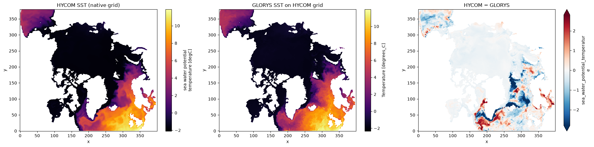
Velocities need rotating to a common frame#
regrid_to_hycom interpolates uo/vo as scalars, so GLORYS velocities land on the HYCOM T-points but stay as geographic eastward/northward components — they are not HYCOM’s native model-axis components on the staggered C-grid. HYCOM’s own u-vel./v-vel. run along the (rotated) model axes, so differencing them against GLORYS directly is wrong wherever the grid turns — i.e. across the whole Arctic cap.
velocities_east_north closes the gap: it de-staggers HYCOM’s velocities to the T-points and rotates them to true east/north using the grid angle pang, keeping the native (y, x) grid. Both fields are then eastward/northward on the same grid and difference directly.
ds["u-vel."].attrs
{'long_name': 'sea water x velocity',
 'units': 'm s-1',
 'hycom_velocity': 'total',
 'comment': 'total current (baroclinic + barotropic); the barotropic part was summed in when the archm time mean was formed'}
# Rotate HYCOM's model-axis velocities to true east/north on the native grid.
hyc = xhycom.velocities_east_north(ds, grid)
hyc["u-vel."].attrs
{'long_name': 'eastward component of sea water x velocity',
 'units': 'm s-1',
 'hycom_velocity': 'total',
 'comment': 'de-staggered to T-points and rotated to geographic axes',
 'standard_name': 'eastward_sea_water_velocity'}
# Both are now eastward velocity on HYCOM's (y, x) grid -> difference directly.
hu = hyc["u-vel."].isel(time=0, k=0)
gu = glorys_on_hycom["uo"].isel(time=0, depth=0)

fig, axs = plt.subplots(1, 3, figsize=(20, 5))
hu.plot(ax=axs[0], cmap="RdBu_r", center=0, robust=True)
gu.plot(ax=axs[1], cmap="RdBu_r", center=0, robust=True)
(hu - gu).plot(ax=axs[2], cmap="RdBu_r", center=0, robust=True)
axs[0].set_title("HYCOM eastward (rotated)")
axs[1].set_title("GLORYS eastward (uo) on HYCOM grid")
axs[2].set_title("HYCOM − GLORYS")
fig.tight_layout()