Working with HYCOM data

Working with HYCOM data#

This notebook walks through common xarray operations on HYCOM output: slicing, regional masking, curvilinear plotting, time-based aggregations, and groupby for seasonal analysis.

We open the archive lazily with chunks={"time": 1} so the examples work on any size of archive without loading everything into memory (see Lazy loading & chunking to learn more about chunk sizes and lazy loading).

import xhycom

GRID_PATH = "/cluster/home/nlo043/NERSC-HYCOM-CICE/TP2a0.10/topo/regional.grid"
DATA_PATH = "/nird/datalake/NS9481K/shuang/TP2_output/expt_02.8/"

# Open the full archive lazily: no data read until .compute()
ds = xhycom.open_mfdataset(DATA_PATH + "archm.2020*", grid=GRID_PATH, chunks={"time": 1})

ds

<xarray.Dataset> Size: 1TB
Dimensions:     (y: 380, x: 400, time: 366, k: 50, ki: 51)
Coordinates:
    lon         (y, x) float64 1MB dask.array<chunksize=(380, 400), meta=np.ndarray>
    lat         (y, x) float64 1MB dask.array<chunksize=(380, 400), meta=np.ndarray>
    lon_u       (y, x) float64 1MB dask.array<chunksize=(380, 400), meta=np.ndarray>
    lat_u       (y, x) float64 1MB dask.array<chunksize=(380, 400), meta=np.ndarray>
    lon_v       (y, x) float64 1MB dask.array<chunksize=(380, 400), meta=np.ndarray>
    lat_v       (y, x) float64 1MB dask.array<chunksize=(380, 400), meta=np.ndarray>
  * time        (time) object 3kB 2020-01-01 00:00:00 ... 2020-12-31 00:00:00
  * k           (k) int64 400B 1 2 3 4 5 6 7 8 9 ... 42 43 44 45 46 47 48 49 50
    dens        (k) float64 400B dask.array<chunksize=(50,), meta=np.ndarray>
  * ki          (ki) int64 408B 0 1 2 3 4 5 6 7 8 ... 42 43 44 45 46 47 48 49 50
Dimensions without coordinates: y, x
Data variables: (12/83)
    montg1      (time, y, x) float64 445MB dask.array<chunksize=(1, 380, 400), meta=np.ndarray>
    srfhgt      (time, y, x) float64 445MB dask.array<chunksize=(1, 380, 400), meta=np.ndarray>
    oneta       (time, y, x) float64 445MB dask.array<chunksize=(1, 380, 400), meta=np.ndarray>
    surflx      (time, y, x) float64 445MB dask.array<chunksize=(1, 380, 400), meta=np.ndarray>
    wtrflx      (time, y, x) float64 445MB dask.array<chunksize=(1, 380, 400), meta=np.ndarray>
    salflx      (time, y, x) float64 445MB dask.array<chunksize=(1, 380, 400), meta=np.ndarray>
    ...          ...
    CO2_wind    (time, y, x) float64 445MB dask.array<chunksize=(1, 380, 400), meta=np.ndarray>
    ECO_bots    (time, y, x) float64 445MB dask.array<chunksize=(1, 380, 400), meta=np.ndarray>
    surface__1  (time, y, x) float64 445MB dask.array<chunksize=(1, 380, 400), meta=np.ndarray>
    surface__2  (time, y, x) float64 445MB dask.array<chunksize=(1, 380, 400), meta=np.ndarray>
    si_u        (time, y, x) float64 445MB dask.array<chunksize=(1, 380, 400), meta=np.ndarray>
    si_v        (time, y, x) float64 445MB dask.array<chunksize=(1, 380, 400), meta=np.ndarray>
Attributes:
    iversn:   23
    iexpt:    28
    yrflag:   3

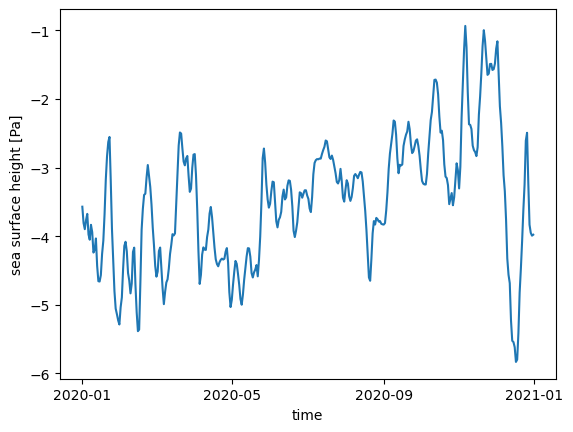
ds["srfhgt"].mean(dim=["y", "x"]).plot()

[<matplotlib.lines.Line2D at 0x1548cf3c69d0>]

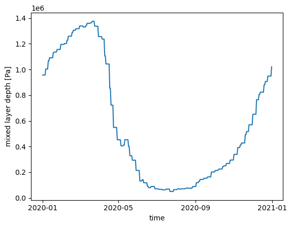
_images/7962acd7761b293c91779aeb0779303d0762f6b6651e8bb3b64e08858610eee5.png

ds["mix_dpth"].mean(dim=["y", "x"]).plot()

[<matplotlib.lines.Line2D at 0x154760a38f50>]

_images/4ea159edc342185c9a77eb2263adfd62836ffa4658f798653432e98294ade557.png

Physical units and derived fields#

By default the data come back exactly as stored on disk, so some fields are in HYCOM’s native units - sea-surface height as geopotential, and layer thickness / mixed-layer depth as pressure in Pa. Pass postprocess=True to convert these to physical units and add a few derived fields:

Field	Native	`postprocess=True`
`srfhgt`	geopotential (m² s⁻²)	sea-surface height in m (÷ g = 9.806)
`thknss`, `mix_dpth`, `bl_dpth`, `thmix`	pressure (Pa)	m (÷ onem = 9806)
`u-vel.`, `v-vel.`	baroclinic (`archv`) / total (`archm`)	total current (+ barotropic), tagged `hycom_velocity`
`area`	-	`scpx · scpy` (m²), on grid files
`landmask`	-	1 ocean / 0 land, from the bathymetry

You can also apply it to an already-open dataset with xhycom.postprocess(ds).

Note

HYCOM writes u-vel./v-vel. differently per file type: an instantaneous archv stores the baroclinic layer velocity, so the total current is u-vel. + u_btrop; a mean archm already stores the total (the barotropic part is summed in online). postprocess=True reconciles both to the total current, adding the barotropic part for archv, annotating archm, and records the provenance in ds.attrs["archive_type"] ("instantaneous" / "mean") and da.attrs["hycom_velocity"] ("total" / "baroclinic"). If you select velocities via variables=, the barotropic u_btrop/v_btrop are pulled in automatically to build the total, then dropped.

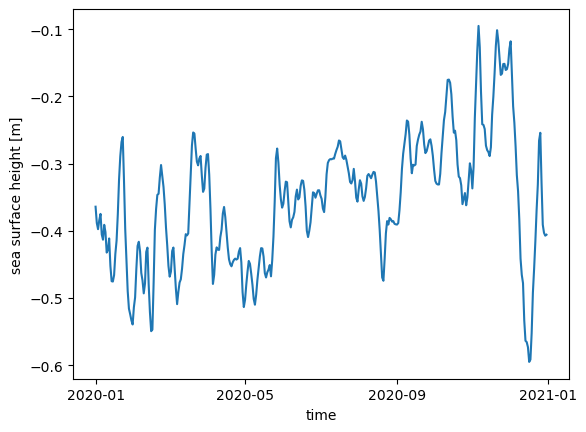
# Same archive with native units converted + derived fields added.
# Kept on a separate handle so the rest of the notebook keeps the raw `ds`.
ds_pp = xhycom.open_mfdataset(DATA_PATH + "archm.2020*", grid=GRID_PATH, chunks={"time": 1}, postprocess=True)

ds_pp["srfhgt"].mean(dim=["y", "x"]).plot()

[<matplotlib.lines.Line2D at 0x1548b0ad3390>]

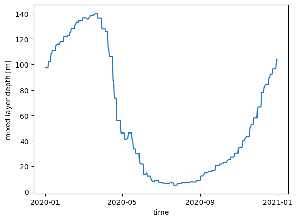
_images/27dd150568ae35a50bb0baafd34ea278cbd77ab171da989e14ea9bf5f720dba7.png

ds_pp["mix_dpth"].mean(dim=["y", "x"]).plot()

[<matplotlib.lines.Line2D at 0x154719edddd0>]

_images/872f215ccdeaa636899da592796805603626f41e83bb34b0bec3082ca583c396.png

# postprocess reconciles u-vel./v-vel. to the total current, and records how:
ds_pp.attrs["archive_type"], ds_pp["u-vel."].attrs["hycom_velocity"]

Slicing#

xarray’s isel (index-based) and sel (label-based) selectors work directly.

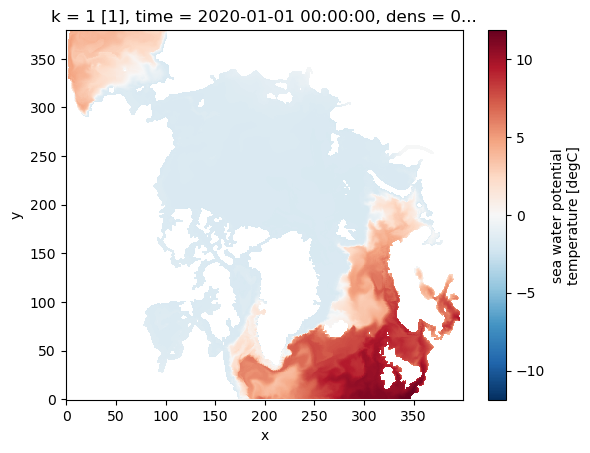
# Surface temperature at the first time step
sst = ds["temp"].isel(time=0, k=0)

sst

<xarray.DataArray 'temp' (y: 380, x: 400)> Size: 1MB
dask.array<getitem, shape=(380, 400), dtype=float64, chunksize=(380, 400), chunktype=numpy.ndarray>
Coordinates:
    lon      (y, x) float64 1MB dask.array<chunksize=(380, 400), meta=np.ndarray>
    lat      (y, x) float64 1MB dask.array<chunksize=(380, 400), meta=np.ndarray>
    lon_u    (y, x) float64 1MB dask.array<chunksize=(380, 400), meta=np.ndarray>
    lat_u    (y, x) float64 1MB dask.array<chunksize=(380, 400), meta=np.ndarray>
    lon_v    (y, x) float64 1MB dask.array<chunksize=(380, 400), meta=np.ndarray>
    lat_v    (y, x) float64 1MB dask.array<chunksize=(380, 400), meta=np.ndarray>
    k        int64 8B 1
    time     object 8B 2020-01-01 00:00:00
    dens     float64 8B dask.array<chunksize=(), meta=np.ndarray>
Dimensions without coordinates: y, x
Attributes:
    long_name:  sea water potential temperature
    units:      degC

sst.plot()

<matplotlib.collections.QuadMesh at 0x1548b2f34390>

_images/7fb5701a6ff6a8c75699f8d4605e373bd1c225881f2964704f67c673505e5d9b.png

temp_at_fixed_dens = ds["temp"].isel(time=0).isel(k=13)

temp_at_fixed_dens

<xarray.DataArray 'temp' (y: 380, x: 400)> Size: 1MB
dask.array<getitem, shape=(380, 400), dtype=float64, chunksize=(380, 400), chunktype=numpy.ndarray>
Coordinates:
    lon      (y, x) float64 1MB dask.array<chunksize=(380, 400), meta=np.ndarray>
    lat      (y, x) float64 1MB dask.array<chunksize=(380, 400), meta=np.ndarray>
    lon_u    (y, x) float64 1MB dask.array<chunksize=(380, 400), meta=np.ndarray>
    lat_u    (y, x) float64 1MB dask.array<chunksize=(380, 400), meta=np.ndarray>
    lon_v    (y, x) float64 1MB dask.array<chunksize=(380, 400), meta=np.ndarray>
    lat_v    (y, x) float64 1MB dask.array<chunksize=(380, 400), meta=np.ndarray>
    k        int64 8B 14
    time     object 8B 2020-01-01 00:00:00
    dens     float64 8B dask.array<chunksize=(), meta=np.ndarray>
Dimensions without coordinates: y, x
Attributes:
    long_name:  sea water potential temperature
    units:      degC

temp_at_fixed_dens.plot()

<matplotlib.collections.QuadMesh at 0x154718008390>

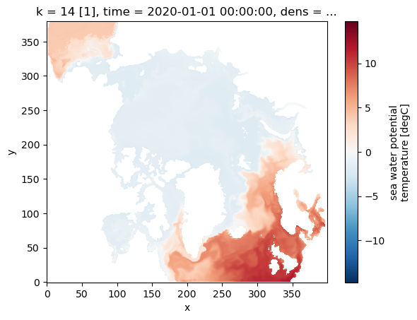
_images/dfe6540d7f2638b8ccef3ca0d1fd55449dd757f82ffb1365459c6eea17da9928.png

# Select by layer density instead of layer index
the_same_temp = ds["temp"].isel(time=0).sel(dens=27.0, method="nearest")

the_same_temp.plot()

<matplotlib.collections.QuadMesh at 0x154903f33d10>

Regional analysis#

HYCOM uses a curvilinear grid, so lon and lat are 2-D arrays, you cannot use .sel(lon=..., lat=...) for spatial subsetting. Instead, build a boolean mask from the coordinate arrays and apply it with .where().

# Boolean mask: True inside the region, False outside
mask = (ds.lon > -30) & (ds.lon < 30) & (ds.lat > 50) & (ds.lat < 80)
mask.plot(cmap='RdYlGn');

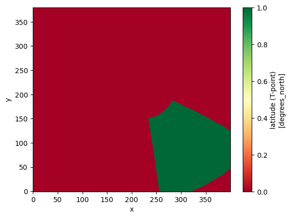
_images/4aec148645001df452d20b8a881fd087f22eed98048d0f8417647eac57c52656.png

Apply the mask to a variable, grid points outside the region become NaN:

sst_region = ds['temp'].isel(k=0).where(mask)
sst_region.isel(time=0).plot();

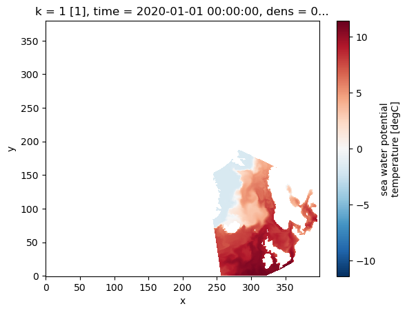
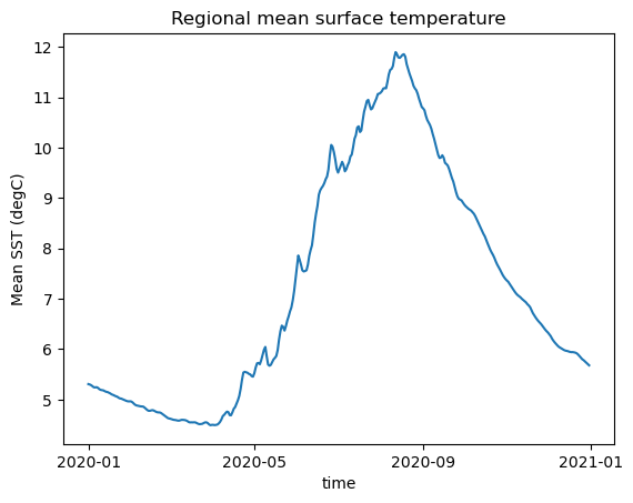
_images/03f66e1bf0e18232c53974ec44070c66a9e60b8d321beb14ac1f9ab539e73183.png

With the mask applied, reductions like .mean() automatically ignore the masked-out (NaN) points. Here we compute a time series of mean surface temperature inside the region:

sst_ts = sst_region.mean(dim=['y', 'x']).compute()
sst_ts.plot()
import matplotlib.pyplot as plt
plt.ylabel('Mean SST (degC)')
plt.title('Regional mean surface temperature');

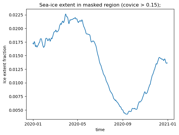
_images/76dc75e0d796f72f378e67215817e4d9c909703b81d8ee6a5adffa69ac9bb8d2.png

The same pattern works for any variable. For example, sea-ice extent (fraction of the masked area with ice concentration above 15 %):

ice_extent = (ds['covice'].where(mask) > 0.15).mean(dim=['y', 'x']).compute()
ice_extent.plot()
plt.ylabel('Ice extent fraction')
plt.title('Sea-ice extent in masked region (covice > 0.15);');

_images/3810e94a6334e822c67e6cb20afa429b0ce6aba861e241b4743adacc64108106.png

Seasonal and monthly analysis with `groupby`#

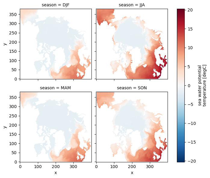
groupby splits the time axis by a label, calendar month, season, year, and applies a reduction. Everything stays lazy until .compute() is called.

# 4-season mean of surface temperature (reads all files on .compute())
sst_seasonal = ds["temp"].isel(k=0).groupby("time.season").mean()
sst_seasonal

<xarray.DataArray 'temp' (season: 4, y: 380, x: 400)> Size: 5MB
dask.array<stack, shape=(4, 380, 400), dtype=float64, chunksize=(1, 380, 400), chunktype=numpy.ndarray>
Coordinates:
  * season   (season) object 32B 'DJF' 'JJA' 'MAM' 'SON'
    lon      (y, x) float64 1MB dask.array<chunksize=(380, 400), meta=np.ndarray>
    lat      (y, x) float64 1MB dask.array<chunksize=(380, 400), meta=np.ndarray>
    lon_u    (y, x) float64 1MB dask.array<chunksize=(380, 400), meta=np.ndarray>
    lat_u    (y, x) float64 1MB dask.array<chunksize=(380, 400), meta=np.ndarray>
    lon_v    (y, x) float64 1MB dask.array<chunksize=(380, 400), meta=np.ndarray>
    lat_v    (y, x) float64 1MB dask.array<chunksize=(380, 400), meta=np.ndarray>
    k        int64 8B 1
    dens     float64 8B dask.array<chunksize=(), meta=np.ndarray>
Dimensions without coordinates: y, x
Attributes:
    long_name:  sea water potential temperature
    units:      degC

sst_seasonal.plot(col="season", col_wrap=2)

<xarray.plot.facetgrid.FacetGrid at 0x15484a405a50>

_images/bcd0af1c119f98c95d74733dcaba49e1459b0f8cfbf672cca868a5c1174e8f0c.png

March sea-ice concentration#

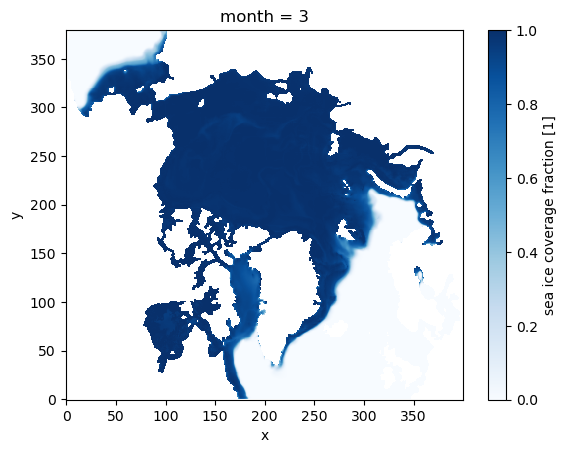
Monthly groupby lets you compute a climatological mean for any specific month. Here we extract March (month 3) mean sea-ice concentration across all years.

# Climatological March sea-ice concentration
ice_monthly = ds["covice"].groupby("time.month").mean()
march_ice = ice_monthly.sel(month=3)
march_ice

<xarray.DataArray 'covice' (y: 380, x: 400)> Size: 1MB
dask.array<getitem, shape=(380, 400), dtype=float64, chunksize=(380, 400), chunktype=numpy.ndarray>
Coordinates:
    lon      (y, x) float64 1MB dask.array<chunksize=(380, 400), meta=np.ndarray>
    lat      (y, x) float64 1MB dask.array<chunksize=(380, 400), meta=np.ndarray>
    lon_u    (y, x) float64 1MB dask.array<chunksize=(380, 400), meta=np.ndarray>
    lat_u    (y, x) float64 1MB dask.array<chunksize=(380, 400), meta=np.ndarray>
    lon_v    (y, x) float64 1MB dask.array<chunksize=(380, 400), meta=np.ndarray>
    lat_v    (y, x) float64 1MB dask.array<chunksize=(380, 400), meta=np.ndarray>
    month    int64 8B 3
Dimensions without coordinates: y, x
Attributes:
    long_name:  sea ice coverage fraction
    units:      1

march_ice.plot(cmap="Blues", vmin=0, vmax=1)

<matplotlib.collections.QuadMesh at 0x15450cfef690>

_images/bf20ea1d0f6adf9260fd639081932e52585581ba965c57efaba81d73284fe66b.png

Anomalies#

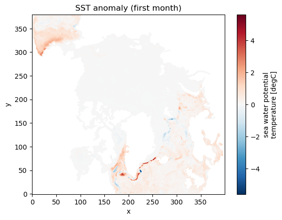
Subtract the climatological monthly mean to isolate interannual or seasonal variability.

import matplotlib.pyplot as plt

# Climatological monthly mean
clim = ds['temp'].isel(k=0).groupby('time.month').mean()

# Anomaly: each time step minus its climatological month
anom = ds['temp'].isel(k=0).groupby('time.month') - clim

# Plot the anomaly for one time step
anom.isel(time=0).compute().plot(cmap='RdBu_r', center=0)
plt.title('SST anomaly (first month)');

_images/05b26e26df90b1e862d0f5c35b1f322310172b248ca908a8c3749dd7acd226e5.png

Mixed layer depth#

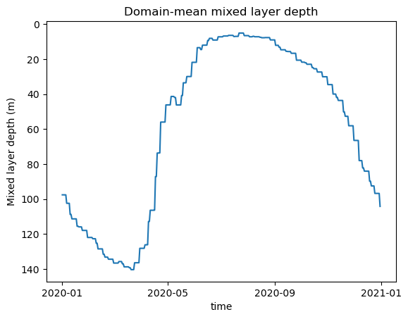
mix_dpth is stored in Pa, divide by ~9806 to convert to metres. (With postprocess=True this conversion is done for you, so ds_pp["mix_dpth"] is already in metres and the manual / 9806.0 below is unnecessary.)

# Mixed layer depth in metres, time series averaged over the domain
mld_m = (ds['mix_dpth'] / 9806.0).mean(dim=['y', 'x']).compute()
mld_m.attrs['units'] = 'm'
mld_m.plot()
plt.ylabel('Mixed layer depth (m)')
plt.gca().invert_yaxis()          # depth increases downward
plt.title('Domain-mean mixed layer depth');

_images/12498785007fc5cd768e02dcf14e8a123bf0e1eb979262f391e5e28b43df8852.png

Saving a subset to NetCDF#

Use to_netcdf() to write a subset of variables or time steps to a file for sharing or use with tools that do not read .ab format directly.

# Write the top 10 layers of T and S for the first 12 time slices
subset = ds[['temp', 'salin']].isel(time=slice(0, 12))
subset.compute().to_netcdf('hycom_TS_2020.nc')
print('Saved hycom_TS_2020.nc')

Saved hycom_TS_2020.nc

Plotting#

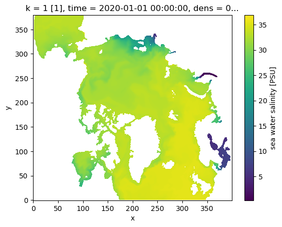
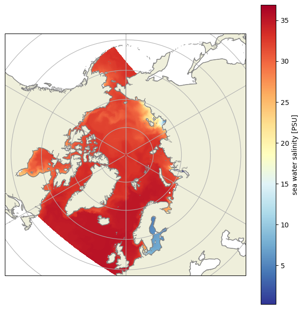
sss = ds["salin"].isel(time=0, k=0)

For quick plots, use xarray’s in-built plotting.

sss.plot()

<matplotlib.collections.QuadMesh at 0x15484a74a150>

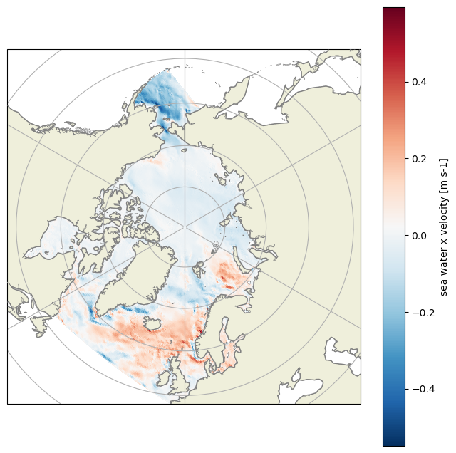
_images/1848ab6358518442a21bdbb1d796b820b02d6dd62e9d3be62bc818ce626070d9.png

Because lon and lat are 2-D curvilinear arrays, use pcolormesh directly rather than xarray’s .plot(). U-point and V-point variables carry lon_u/lat_u and lon_v/lat_v coordinates.

import matplotlib.pyplot as plt
import cartopy.crs as ccrs
import cartopy.feature as cfeature
import numpy as np

def ArcticMap():

    fig, ax = plt.subplots(
        figsize=(8, 8),
        subplot_kw={"projection": ccrs.NorthPolarStereo(central_longitude=0.0)},
    )

    ax.set_extent([-180, 180, 48, 90], crs=ccrs.PlateCarree())
    ax.add_feature(cfeature.LAND, facecolor=cfeature.COLORS["land"], edgecolor="grey", zorder=2)
    ax.add_feature(cfeature.COASTLINE.with_scale("50m"), edgecolor="grey", linewidth=0.4, zorder=3)
    ax.gridlines()
      
    return fig, ax

def pcolormesh_curvilinear(lon, lat, data, ax=None, **kwargs):

    proj = ax.projection
    pxy = proj.transform_points(ccrs.PlateCarree(), lon, lat)
    px, py = pxy[:, :, 0], pxy[:, :, 1]
    invalid = ~np.isfinite(px) | ~np.isfinite(py)
    px = np.where(invalid, 0.0, px)
    py = np.where(invalid, 0.0, py)
    data = np.where(invalid, np.nan, data)
    return ax.pcolormesh(px, py, data, **kwargs)

fig, ax = ArcticMap()
p = pcolormesh_curvilinear(sss.lon.values, sss.lat.values, sss.values, ax=ax, cmap="RdYlBu_r")
fig.colorbar(p, ax=ax, label=f"{sss.attrs['long_name']} [{sss.attrs['units']}]")

<matplotlib.colorbar.Colorbar at 0x15451b6a2bd0>

_images/2d79f94214d0b204e7f912a52f9c3f38bdf8e391a4bb2f07670829bfa261ed68.png

u = ds["u-vel."].isel(time=0, k=0)

# U-point variable: use lon_u / lat_u

fig, ax = ArcticMap()
p = pcolormesh_curvilinear(u.lon_u.values, u.lat_u.values, u.values, ax=ax, cmap="RdBu_r")
fig.colorbar(p, ax=ax, label=f"{u.attrs['long_name']} [{u.attrs['units']}]")

<matplotlib.colorbar.Colorbar at 0x1546fceeb410>

_images/06668a11bb5e87bcb2bc3d7f8c6d40d92646fffbb270b653b47daa9682d316b4.png